| All postings by author | previous: Emitter arrays | up: Three types of waves | next: next blog |
Wave-centric interpretation of quantum mechanics
by Peter H. Ceperley
Keywords: interpretation of quantum mechanics, wave-centric, real waves
Alternate location: Mason Archival Repository Service
Table of contents
1. Summary
This paper explores one interpretation of quantum mechanics: that perhaps the waves of quantum mechanics are real and the particles, i.e. the quanta, are merely properties of atoms, the atoms which are responsible for launching and absorbing the waves. In this interpretation, the waves of quantum mechanics are emitted in discrete quanta, but after emission they spread out as waves do. A detector's atoms are continuously bathed in a sea of zero point noise which is in equilibrium with these atoms. An outside wave, even if faint, will throw off this equilibrium which results in one or more atoms in a particle detector absorbing a quantum partially from the wave and partially from the zero point noise field. In this article we show that the number of atoms absorbing a quantum will be proportional to the energy density of the external wave.
2. Introduction
All things in quantum mechanics propagate as waves but are emitted and absorbed as particles.
In quantum mechanics all entities are considered to have both particle-like and wave-like attributes. This is often summed up as: entities propagate as waves but are emitted and absorbed as particles. The standard interpretation of quantum mechanics, i.e. the Copenhagen interpretation, puts more emphasis on the particle side, implying that these tiny entities are basically particles but somehow magically propagate as waves. The current paper explores the obvious other interpretation, that elementary "particles" really are waves, not particles, but these waves are emitted and absorbed in such a way as to mimic particle emission and absorption. For other, non-conventional interpretations see wikipedia.
The particles: In this paper the "particles" that we wish to consider as waves are those truly elementary particles that are not composites of smaller entities. Possibilities are electrons, quarks, photons, phonons, etc. Composites such as atoms are localized entities, i.e. particles, that are composed of waves internally. We will put off dealing with composites to a future paper. While we will not be concerned with atoms as particles (as in interfering beams of atoms), we will be very interested in them playing another very important role as wave emitters and absorbers as discussed in Section 3 below.
The waves: We envision these waves to be fairly complicated, similar to the waves that can exist in some solid state materials so as to allow the waves to carry properties that are conventionally associated with elementary particles. That is to say that electron waves will carry charge and spin. The spin aspect would be similar to spin waves that exist in magnetic materials. Quark waves would be even more complex with more properties in the waves. Viewing elementary particles as waves amounts to assuming that space is a medium that supports these various complicated waves. The inclusion of charge as a wave property makes electron and quark waves non-linear; that is, the wave trajectories, wavelength, etc. can depend on the amplitude of the waves.
The atom: In this interpretation an atom is considered to have a central positive core which traps electron waves in various excitation modes, i.e. orbitals. Thus atoms are solitons of a sort. The non-linearity of the waves opens up the possibility that stable electron waves in an atom only exist at one select excitation level for each mode. If we assume such discrete excitation levels then whenever a mode is to be excited, an atom will absorb one quantum of energy and when it radiates energy, it will radiate one quantum of energy. This makes absorption and emission of radiation occur in quanta. We deal more with absorption in the next section.
Emission: If an atom emits a quantum of electromagnetic energy or an electron, that wave will spread and flow outwards away from the atom in a normal wave fashion as dictated by the Maxwell or Schroedinger equations modified to carry spin and charge as appropriate.
3. Absorption
In quantum mechanics "measurements" are the only way we know what is happening. That is to say we envision quantum mechanical waves propagating here and there but until we make a "measurement" we can be sure of nothing. But a measurement is a drastic step because in the conventional interpretation when a measurement is performed, the waves, spread out as they may be, instantaneously collapse onto the site of the measurement and propagate no more. The instantaneous collapse violates relativistic causality, but is accepted as one of the mysteries of quantum mechanics.
| Examples of “measurements” |
|---|
|
What constitutes a measurement? Our view is that a “measurement” consists of absorption of the wave by an atom. (See examples listed at right.) Whenever an atom absorbs a quantum mechanical wave and undergoes a change as a result, we can, if we choose, deduce something about what the quantum mechanical wave was doing before the absorption. The atomic absorption scrambles the quantum mechanical wave and is usually considered irreversible, that is, the initial wave cannot be reconstructed.
Just how does the spread out wave field concentrate itself to allow one quantum of energy or a whole electron to be absorbed by an atom? As we stated above, the conventional interpretation resorts to magic to explain this effect. In the wave-centric interpretation we hope to get rid of the magic and restore causality to the understanding of quantum mechanics.
In the wave-centric interpretation, absorption can be explained in terms of a background noise, most likely the zero-point energy. In this interpretation we assume there is an undetectable noise field filling space in equilibrium with the atoms. This is in addition to any thermal (temperature related) noise. This noise field is undetectable because we interpret zero point effects as due to quantum mechanics.
In the next section we will show that a noise field which provides energy around and available to every atom can cause the quantum mechanical particle-like energy absorption. This does not mean every particle will see the same level of noise energy at all times. Being chaotic as noise fields are, at any instant around some atoms there will be more noise energy and around other atoms there will be less noise energy. It is also true that at any instant the noise around some atom will be phased just right to best add to whatever external wave is arriving. If no external radiation is present, this noise will be in equilibrium with the atoms and will result in very few if any actual transitions.
When there is an external wave present and this wave combines with the noise field, some lucky atom or atoms will be in just the right place and have just the right phase to use the noise energy plus the external radiation to absorb a quantum and make a transition. During the transition, the atom will, as all wave receivers do, emit a canceling wave which will cancel the nearby combined noise and external wave fields and thereby deny other nearby atoms the opportunity to make a transition. This emission of a canceling wave allows the atom to have an effective cross section for absorption much, much bigger than its physical size. This is the same effect that also allows small AM and FM radios to similarly have a very enhanced absorption cross section, again much larger than their physical sizes.
The larger the external wave is, the more atoms will happen to have sufficient surrounding noise fields to allow them to effect a transition. If we count each transition as a "particle" then we will "detect" (via transitions) more "particles" in regions of stronger external wave fields. In the next section we do the math to derive the distribution of noise amplitude required to make the number of transitions be proportional to the energy in the external wave.
To summarize absorption: the wave-centric interpretation hypothesizes that atoms are surrounded by a noise field and that this noise field allows even weak external waves to cause an occasional atomic transition as expected in quantum mechanics. We might view the atoms as popcorn kernels on a hot frying pan just waiting for an extra bit of heat to make them pop; the stronger this "external heat" the more kernels will pop.
4. Required distribution of noise amplitudes:
In this section we assume a triangular distribution of noise amplitudes. We then go on to show that this results in the probability of a detection being proportional to the external wave energy. We also show that random phases in the various waves making up the noise result in a total amplitude having a distribution that is nearly triangular.

|
| Fig. 1.Triangular noise distribution. This curve shows the probability (per amplitude) that noise will be able to impart a given amplitude to a resonator (such as an atom). Later we will explore possible sources of this noise distribution. On the horizontal axis is the component of noise amplitude that is in phase with a particular external wave. Negative noise amplitudes indicate that the noise is phased to subtract energy from the atom. We will be primarily interested in the right half of the distribution which has has a total probability of one (area under the right side of the distribution). |
Suppose we pick a point at which to examine the noise and repeatedly measure the noise amplitude at this point over a period of time. Because of the ever changing nature of noise fields we expect to see a variation in amplitudes of our measurements. This variation is due to the mix of waves in the noise field having various frequencies and beating with each other. The resulting time-varying field will, at times, add to any particular external wave and at other times will subtract from it.
Triangular noise distribution: Fig. 1 shows a triangular noise amplitude distribution. This represents one possible distribution of amplitudes. It shows the relative fraction of time a certain amount of noise amplitude will be available to an atom for the purpose of making a transition.For convenience, we assume amplitude units such that an amplitude of +1 (plotted on the horizontal axis of the graph) is the amplitude required to cause a transition without any external wave. According to the graph in Fig. 1, there is zero probability of such a +1 amplitude.
At this point in our explanation we are only interested in positive amplitudes, those which will potentially add to a particular external wave's amplitude and be involved with a quantum absorption. These positive amplitudes are on the right side of Fig. 1. We can express the linear region on the positive side of Fig. 1 as:
![]() . (1)
. (1)
For larger noise amplitudes where Anoise > 1 , the probability P1 = 0 .
Resulting transitions:
We need to determine the probability that the noise as specified in Fig. 1 will be available to participate in a transition. That is, given an external wave of amplitude Aext , we need to calculate the probability that the sum of the noise amplitude and the external wave amplitude will be greater or equal to the amplitude for a transition.
For this we need the probability P2 that the noise will be greater or equal to a given minimum value Amin . This can be calculated from (1):
 .
.
Doing the final evaluation, we get:
![]() , (2)
, (2)

|
| Fig. 2. Parabolic noise distribution. This is the shape of the noise amplitude distribution when the horizontal axis represents the minimum amplitude. |
which we plot in Fig. 2.
In Fig. 3 we have changed the horizontal axis from the minimum noise amplitude into the external wave amplitude required to make the total amplitude available to the atom to be equal to or greater than +1 (i.e. one quantum). That is to say such that Amin + Aext = +1 .
We can turn this last equation around and solve for the amplitude of the external wave, i.e. Aext = 1 − Amin . Looking at Eqn. (2) we see this makes the probability
P2 = (Aext)2 . (3)
Thus we now have the probability of transition as a function of the amplitude of the external wave, as plotted in Fig. 3 below.
Equation (3) indicates that the transition probability equals the external wave amplitude squared. We know that the wave energy Eext is also proportional to the wave amplitude squared. We can now write:
P2 ∝ Eext . (4)
Thus the probability of detection is proportional to the energy of the external wave as shown in Fig. 4.
This is consistent with conventional quantum mechanics. Note again that this is for a background noise with a triangular amplitude distribution as shown in Fig. 1 . As a final cross check we note that Fig. 3 shows that an external wave with an amplitude of +1 which we defined earlier to be equivalent to one quantum (available energy to an atom) which will have 100% chance of causing a transition.

|

|
| Fig. 3. Probability of transition versus amplitude of external wave adding to the noise amplitude. | Fig. 4. Probability of transition versus external wave energy. |
5. Distribution resulting from random phases incident on atoms:

|
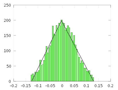
| Fig. 5. Typical histogram showing the frequency of occurrence of various total amplitudes resulting from summing many waveforms with random phases, frequencies, and amplitudes. The waveform amplitudes were multiplied by a resonator response function. Also shown is a fitted Gaussian distribution. |
We used Octave to calculate the distribution of amplitudes of a particular phase (to match the phase of a specific external wave) that might be expected in a linear resonator (our atom). We summed waves with random phases, amplitudes and frequencies. Fig. 5 shows the resulting distribution with a fitted Gaussian. We see the fit is good.
Fig. 6 shows a Gaussian as compared with a triangular distribution. The two curves differ at the peak around Anoise = 0 and also around the edges, i.e. around Anoise = ±1. If an atom did experience an amplitude with an absolute value greater than 1, this amplitude would cause a transition without any extra outside wave. This means that the atom would instantaneously absorb all the amplitudes with an absolute value in excess of 1 and leave small amplitudes remaining. The small amplitude "clippings" would add to the center part of the distribution curve making the Gaussian more triangular as shown in Fig. 7. As we can see the results are a nearly triangular amplitude distribution. A better modeling of this process would require modeling of the atom as a non-linear resonator surrounded by a noise field which is in equilibrium with other non-linear atom/resonators. Hopefully with more complete modeling a truly triangular noise distribution would be achieved.

|
|
| Fig. 6. Comparison of triangular and Gaussian distributions. | Fig. 7. Result of clipping amplitudes outside the ±1 quantum region to crudely simulate atoms quickly absorbing one quantum of these amplitudes. The remains of these clippings are added to the distribution increasing the center peak region. Also shown is a fitted triangular distribution (in black) which now is a moderately good fit. |
6. Questions and brief answers concerning specific applications of the wave-centric interpretation
- What about particle tracks such as those in a cloud chamber? Are these not very compelling evidence that there really are subatomic particles? Answer: these are just as much compelling evidence that there really are waves. As explained many years ago [see Schiff, Quantum Mechanics, 2nd Ed. p.209-210, McGraw-Hill 1955] each spot on a cloud chamber or bubble chamber, etc is due to an atomic absorption or excitation and results in the collapse of the wave function (or atomic transition in our interpretation), a re-concentrating of the energy and a re-emission of most of the energy in the direction of momentum. This re-concentration makes it extremely likely that another measurement event will happen just down stream from the first, and that will result in another re-concentration and re-emission, and so on, resulting in a trail of events, i.e. a track. The tracks are due to successive ``measurement" events of the waves and not necessarily due to the presence of a localized particle. In the wave-centric interpretation zero point noise is integrally involved in each measurement.
- Which-way experiments
have been popular in the last several decades. In these a non-linear
element splits a very dilute beam of photons and sends the two halves on
different paths which eventually recombine at a detector which sees an
interference pattern of one type or another. The beam is made dilute
enough so that there is only one photon in the setup at a time. If we
add a detector along one path to try to determine which path a
particular photon is traveling, the interference pattern goes away.
Since conventional quantum mechanics considers a single photon
unsplittable it is not clear how a single photon can sample both routes
and interfere with itself. It is also unclear how a single photon knows
when a detector is placed in the path it doesn't take.
Answer: In the wave-centric interpretation, there are actual waves traveling both routes simultaneously and they recombine and interfere at the final measuring point as waves would. If we block the waves in one path with an additional measurement device, the interference is destroyed just as it would be in classical wave experiments. If we partially block a path, the interference is reduced.
- What about quantum entanglement experiments? In these experiments twin
pairs of "particles" are produced and separate. Before measurement,
these particles can have a wide range of properties. Measurement of one
particle seems to fix the properties of the other particle
instantaneously even if the two are separated by very large distances.
These experiments are cited as proof that quantum mechanics is strange
and cannot be explained by a deterministic interpretation.
Wave-centric answer: Most likely any particular pair of wave packets sent out were a lot more limited in space, time and/or other properties than many physicists assume, even though the ensemble of all the particles (i.e. all the wave packets) under consideration involve greatly varying properties. For example, consider the decay of positronium which often results in two oppositely traveling gamma rays. Probably the wave packets of a specific pair of "photons" were directed oppositely along a specific axis during creation due to the internal dynamics of the decay process. It is then no mystery that later detection of the two would reveal them to be traveling in opposite directions.
- Bell's hidden variable theorem. This applies to particles trying to mimic waves. We are proposing that only waves carry all the measurable properties. This purely wave approach is not in conflict with Bell's theorem.
- Electron-electron collisions. Our model would set up the calculation with two uniform electron waves colliding with each other. With no tiny particles of very localized strong forces how can we have large angle scattering? This is also a question in conventional quantum mechanics. In conventional quantum mechanics we convert to a center of mass reference frame then proceed to calculate the results of two quantum mechanical plane waves passing through each other. This wave math would be the same as in the wave-centric approach. In both, the specifics of the quantum mechanical wave equation lead to a certain amount of large angle scattering.
7. Conclusion
In this article we have briefly examined the possibility that the waves in the wave-particle duality of quantum mechanics be elevated to "real" and the "particles" be considered as artifacts of the way the waves behave. More specifically we show that waves in the presence of zero point noise could be responsible for the particle-like aspects of electrons, photons, etc. Unlike the conventional Copenhagen interpretation, the interpretation presented here has the advantage of preserving causality. At the same time, this interpretation needs a lots of additional refinement, extension and detailed modeling.
| All postings by author | previous: Emitter arrays | up: Three types of waves | next: next blog |