In the previous chapter we were considering the following infinite series equations for the functions ex, sinx, and cosx.
Since these were central to Euler's inventing imaginary numbers, perhaps we should examine the series in more detail. Here we look at the terms in the series, one by one. Since the expression for ex has more terms, we will start with the terms in that series.
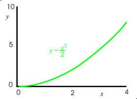
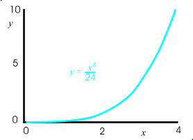
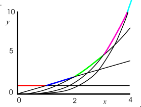
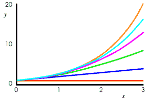
The figures below are graphs of these terms versus x. The last image is that of all the terms or graphs superimposed together. In the last graph, I have colored the region of each where the particular term dominates, i.e. where it is larger than the other terms, that is, has a greater y value.
|
Looking at the last graph above, we see that the first term is largest for small x's, since it starts off at 1 whereas the other graphs start at zero. For a little larger value of x the second terms, the linear term, that grows at a constant rate, dominates. At still a larger x the parabolic curve, i.e. the third terms is largest. It starts off at zero and even has an initial slope of zero, but its higher power law dependence allows it to eventually become the largest. The same is also true for the third and four terms, the higher the power, the larger value of x is required for that term to dominate, but it eventually does. It is also true that we are dividing the higher power terms by a larger constant, sort of handicapping them, to initially stunt them, but eventually their higher power overcomes this effect and they dominate.
When we use an infinite series to represent a function like a sine, cosine, or exponential, we are using this feature, that different power terms can be made to dominate over different parts of the graph. We can choose the signs (the +'s or −'s) and the constants in front of the terms to adjust the effect of each term to make the series behave just like the function we are "fitting".
Fitting the Exp Function
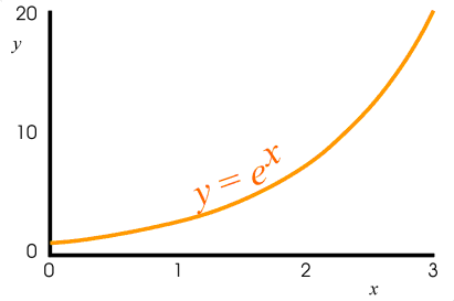
We are first going to use this method to "fit" the exponential function y = ex shown below. This function is famous for eventually reaching greater values than any power law function can. "Exponential growth" of a population or consumption has come to mean an ever increasing rate growth, named after the properties of this function.
| 
|
In the series of graphs below, we see the effect of using one term, then two terms, then three terms, etc. to "fit" the exponential function, which is also shown on each graph.

| 
| 
|

| 
| 
|
In the first graph, only the initial value is matched by the fitting curve, or constant expression. In the second curve, the initial value and the initial slope are both matched and the fitting function now slopes upwards. In the third graph, the initial value, the initial slope, and the initial curvature are are matched and the fitting curve now curves upward in loose approximation to the exponential function. Adding two more terms additionally fit the initial rate of change of the curvature and the rate of change of the rate of change of the curvature. These are actually calculus methods, and the resulting series is called a Taylor series. From the above graphs, we see, that the more terms, the better the fit and the longer the region over which the series fits the function. Adding even more terms to the series would make the fit still better.
The last graph above superimposes all the other graphs, so that you can better compare them.
Calculators and computers often use infinite series as a way to calculate functions, such as sines, cosines, other trigonometric functions, exponentials, logarithms, and square roots.
Fitting the Sine Function
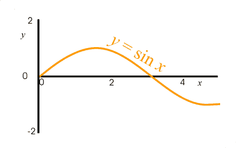
We next turn our attention towards the sine function. Whereas the exponential function was ever increasing, much like most of the terms in the series, the sine function does not resemble the terms, but instead simple undulates between +1 and −1, much like a wave or a snake might do. Below we see the short section of a sine function. As we have seen before, over a much larger range of x values, the repeating, wave-like nature of the sine function is more evident, however here we shall focus on this shorter section.
| . | 
|
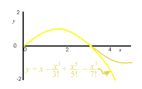
Below we see the fit to the sine function of one term in the series, two terms, three terms, four, and five terms. The series
is a little different from the exponential series above in two obvious ways.
- First, only odd powers are in the series, i.e. only powers of 1, 3, 5, 7, etc.
- Secondly, the signs (the +'s and −'s) between the terms change for each consecutive term, as opposed to the use of only +'s in the exponential series above.
The use of odd powers is a result of the sine function having odd symmetry about the y axis. That is, it is a mirror image of itself flipped over. As a result, the series will only use terms that also have this odd symmetry, i.e. those having the powers of 1, 3, 5, 7, etc.
The alternating signs make this series an "alternating series". It means consecutive terms partially cancel each other and prevent the sum from becoming too large. The use of both positive and negative terms allows us to fit the undulating sine function.

| 
| 
|
| 
| 
|
- The explanation mark in some of the equations on the graphs is a short hand notation for factorials which are a set of consecutively decreasing numbers multiplied together. That is 3! ≡ 3 × 2 × 1 = 6 and 6! ≡ 6 × 5 × 4 × 3 × 2 × 1 = 720, and so on.
- As before, as more and more terms are included, the series fits the sine function better and better, and over a longer span of x values.
- In a computer or calculator program calculating the sine of a number, the series would probably only be used in the range of 0 to 45 ° and other steps in the program would reduce the actual angle to the equivalent angle in this range, over which it is easy to use 5 to 10 terms in the series to obtain outstanding accuracy. For angle in the range of 45 to 90° the program would use the relation that sin x = cos(90° − x) and use the series for cosine discussed next. Because of the use of an alternating series, we have an easy indicator of the error in the approximation. The error will be less than the next term evaluated at the value of x at which we want to know the error in the fit.
Fitting the Cosine Function
We next fit the cosine function, which is very much like the sine function, except that it is shifted over by 90 degrees, i.e π/2 radians. Because of this shift, the function has even symmetry (is a mirror refection of itself on either side of the x axis, and the resulting Taylor series for the cosine is composed only on even powers of x. As listed at the start of this discussion the series is:
Like the sine expansion above, this expansion is an alternating series, where the signs reverse for each consecutive term.

| . | 
|
Below we see a series of graphs of the fit to the cosine function of one term in the series, two terms, three terms, and so on. As before, the more terms, the better the fit and the long the range of x values over which the fit is reasonably good.

| 
| 
|

| 
| 
|
Next: the technology of oscillations and waves demands new mathematical methods.
© P. Ceperley, 2007.
| Good references on WAVES | Good general references on resonators, waves, and fields |
|---|---|
|


