Sines, Cosines, and Phases

We have seen in the last two postings that a Fourier series is intimately linked to sines and cosines. In the last posting we also discovered that there are two forms of Fourier series using sines and cosines.  One form uses cosines with phases and one form uses sines and cosines without phases.  In this posting we will explore this concept in more depth.  

Addition of functions

Animation illustrating the step-by-step process of adding two functions. This shows the laborious process of adding the functions together at each x-position. Mouse over the animation to start it, off to suspend it, click to restart.  You can also use the buttons at the top. You might explore the various functions.   Some may serve to illustrate this idea better for you. copy animation fair use policy

Fourier series involves addition of functions. Mathematically we might express such an addition as:

        .    (1)

This means that for each x, we add the first function's y value at this x to the second function's y value at the same x.  This gives us the sum function's  y value for this x.  

While this is easy to express as an equation, it is rather exhausting to actually do in practice. The animation at the right illustrates this for a number of functions. Mouse and click on the animation to start it. Mouse over the fast button to speed it up, or click on the step button to have it go a step at a time.  Read the caption at the bottom for a step-by-step explanation. Clicking "change f1" or "change f2" will change the functions used. Clicking on the animation will restart it.

The animation shows three functions: a red one on the top graph, a blue one on the middle graph, and a purple one on the lower graph.  The animation shows the process of going point-by-point to sum the upper two functions to make the lower, sum function.

The first set of functions in the animation consists of two sinusoids of the same wavelength. A little observing of the animation will show you that the addition of two same wavelength sinusoids results in another sinusoid of the same wavelength. This concept is a very important point in this posting.  

Relationship between sine and cosine functions

As was briefly explained in the last posting, the sine and the cosine functions are very similar. The two are shown in the graph at the right. The sine function is identical to the cosine function except that the sine function is shifted to the right by 90°.  Another way to achieve a 90° right shift is by subtracting 90° from the argument of the cosine function, i.e. using cos(θ − 90°) in place of cosθ  (you can use this method to shift any function over... subtract a constant from its argument).  We would call this a −90° phase shift.  Or alternately, we can say that the cosine function is a sine function shifted  90°, i.e. to the left.  There are many references on the internet for the relationship between sines and cosines (google on "trig identities").  The equations for the relationships used here are:

sinθ = cos(θ − 90°) cosθ = sin(θ + 90°)

(2)

As was mentioned in the last posting, we can add mixtures of sine and cosine functions together to produce a cosine with various amplitudes and phases.  The animation below illustrates this.  The red and blue functions are cosine and sine functions, respectively, each multiplied by an expanding or reducing coefficient.  The sum of the two functions is shown in purple.  The purple function can be arrived at by adding the two functions together, x position by x position, or by using phasors, as is shown on the right side of the animation.  The viewer can drag the squares of the sine and cosine functions to experiment with changing the amplitudes of these functions.  The viewer can also drag the amplitude and phase of the sum function and see what sine and cosine amplitudes are required to produce various combinations of amplitude and phase.

The backgrounds of the graphs are colored red and blue to indicate the regions of the sum function that are dominated by either the red cosine function or the blue sine function.  The phasor dial is a graphical way to represent the phase of the functions, similar to the way the phase of the moon is represented on some clocks. The use of phasors to add sinusoidal functions is explained (and animated) in the earlier posting titled "phasors". Look at the paragraph titled "Adding two waves in a phasor diagram".

Animation showing how sine and cosine functions with adjustable amplitudes can add up to form a cosine function with any amplitude and phase. Both the functions and their phasors are shown.  The user can drag the handles (small colored squares) to adjust the amplitudes of the sine and cosine functions and see the result of their summation.  Or the user can adjust the amplitude and/or phase of the sum function and see the changes in amplitudes of the sine and cosine functions necessary to produce this sum function.  Alternately, the user can adjust the phasors to accomplish the same results. You can also type in different values in the equations (hit "enter" after making the change.) You might try dragging the purple sum function handle in the left graph horizontally and observe the movement of the phasor. Or, observe how the pure sine and cosine functions rise and fall as needed to accommodate the changing phase. copy animation fair use policy

The mathematical relationships between the amplitudes of the sine and cosine functions and the amplitude and phase of their sum are:

(3)
(4)	(5a)  (5b)
(6)	(7)

The first equation simply states that the cosine function with amplitude A₃ and phase φ is the sum of cosine and sine functions with respective amplitudes A₁ and A₂.  In a sense it defines the constants A₁,  A₂, A₃, and φ.  We use the independent variable θ  here but other variables could easily be substituted for θ, such as x.  The second line of equations gives the amplitude and phase of the sum in terms of the amplitudes of the cosine and sine functions.  Note that the phase φ is best given in terms of the arctan2 function, as seen in many programming languages, which returns angles over the entire 360° or 2π radians. The third line of equations gives the inverse of the equations in the second line, the amplitudes of the sine and cosine functions required so that they sum to a cosine function with amplitude A₃ and phase φ. These relationships are derived in the box below at the right.

Derivation of the relationships in the previous table

We start with the standard relation for the cosine of the sum of two angles:   Applying this to the left side of equation (3) in the previous table, we have:     Comparing this with the right side of equation (3), we see that the first term in parenthesis is the coefficient of cosθ or A1, i.e.   A1 = A3 cos φ    which is equation (6) above.   The second term in parenthesis (the coefficient of sinθ) is, according to equation (3),  A2 so that A2 = −A3 sin φ      which is equation (7).   Now we use our just proven equations (6) and (7).  To get equation (4), we simply square both sides of equations (6) and (7) and add them together:   , or   where in the last step we have used the fact that the sine squared (of any variable) plus the cosine squared (of that same variable) equals one.  We solve the last expression for A3 to give us equation (4).   We get equation (5) by dividing equation (7) by equation (6) and canceling out the A3's that are in both the numerator and the denominator of the right side.  We then apply the inverse (i.e. arc) tangent of both sides.

Relationship of the above formulas to the two forms of Fourier series

In the last posting we presented the following two versions of Fourier series:

(8),

(9)

These two versions are related to each other via the equations (3) through (7) above.  Of course we need to change the variable names of the amplitudes and also replace θ with nθ.  Equation (3) shows the overall relationship that allows us to change equation (8) into equation (9), whereas equations (4) through (7) show the relationship between the amplitudes and phases in equation (8) and equation (9).  Changing the names of the amplitudes as appropriate and replacing θ with nθ, we have:

(10)
(11)	(12a)  (12b)
(13)	(14)

As we said in the previous posting, version (8) of the Fourier series equation is easier to understand, while version (9) is a much easier form to compute the coefficients for, if we are given a function.  Equations (11) through (14) allow us to convert one version into the other.  

Review of the example done in the last posting:

At the end of the previous posting we computed the coefficients for version (9) using the standard equations at the left below on the waveform shown in the center below:

Equations, waveform, and results of the previous posting's example.
(15)
(16)
(17)

We obtained the result that the constant term a₀ was ½.  All the cosine terms were zero, i.e. all the a_n's equaled zero.  Also half the b_n's were zero as well (those with even n numbers).  The odd  sine terms had coefficients given by:  b_n = 2/nπ and are graphed in the right-most panel above.

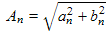
Using equation (11) with these a's and b's, we see that the amplitudes, the A_n's,  are given as follows:  for even n's, A_n = 0 while for odd n's A_n = 2/nπ.  Using equation (12), we see that the φ_n's for even n's are indeterminate (they equal 0/0), while for odd n's the phase shifts are given by φ_n = −π/2 .  

The A_n's are the amplitudes of the various Fourier components while the φ_n's are the phase shifts. For this particular function, a graph of the A_n's versus n would look exactly like the right panel above, except that the vertical axis would be labeled A_n and not b_n.

Repeating the exercise with a shifting of the function:

For another example, consider shifting the waveform above, so that now it is symmetrically placed on either side of the y axis, as show at the left below.  We use integration from 0 to 2π as we did in the previous example, but we could equally well have integrated from  −π to +π and gotten the same results.  This might be a good exercise for a student to try.  The rule is that you need to integrate over exactly one cycle of the repeating waveform.

Example 2.  Symmetrical square wave.
Function to be broken into Fourier components	Calculation of the constant term
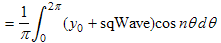
Calculation of the cosine coefficients	Calculation of the sine coefficients
or

The cosine coefficients for example 2.  Note that they alternate in sign.

Looking at the above results, we see that the constant term is still one half.  This is as we would expect, since  the average value will remain unchanged during a simple shifting to the right or left. However the other coefficients, the a_n's and b_n's, do change.  In our new case, the sine coefficients, the b_n's, are all zero and the cosine coefficients, the a_n's, are the same as the sine coefficients of the previous example, except that they now alternate in sign.  Shifting over has interchanged the values of these two sets of coefficients and added the ± sign. Someone experienced with Fourier series would say a lot of this is obvious, that after subtracting the constant term, the first example is an anti-symmetric function ( f(−θ) = −f(θ) ), while the second example is a symmetric function ( f(−θ) = f(θ) ).  To an experienced person, this would mean that the sinusoid components in the first case would be anti-symmetric, i.e. sine functions, while those in the second case would be symmetric, i.e. cosine functions.  

If we use equations (11) and (12), we find that the A_n's are just as before:  A_n = 0 for all even n's and A_n = 2/nπ for all odd n's.  On the other hand, the phases have changed:  while the φ_n's for even n's are still indeterminate, the φ_n 's for odd n's alternate between 0 and π   (i.e. φ_n = 0 and π).  In the previous example φ_n = −π/2.  Thus, the phases have changed.

As a general rule, shifting a waveform in the horizontal direction does not change the A_n's but it does change the relative sizes of the a's and b's and the phases, the φ_n's.   Although we haven't demonstrated this here, it is also true that shifting the function vertically only changes the constant term a₀ and not the other coefficients, the a_n's and b_n's. An interesting exercise for students is to try this, i.e. add the constant 2 to the above function and redo the calculations.

The following table summarizes the comparison of examples 1 and 2.

Comparison of examples 1 and 2
	Example 1 square wave↓	Example 2 - symmetric square wave -  shifted↓	Comparison↓
Function to be analyzed →			Example 2 is shifted to the left, i.e. by a phase of + radians.
Spectrum →			The two spectra are the same.
Phases → Concerning the labeling of some phases as "indeterminate" (n's for which An = 0, i.e. zero amplitude). Equations (13) and (14) above indicate that zero amplitude (An = 0) means that an = bn = 0. Substitution into equation (12) yields an indeterminate φn. In terms of phasors, this is equivalent to saying that a phasor (or vector) with zero length has an indeterminate direction.	n φn 1 −π/2 2 indeterminate 3 −π/2 4 indeterminate 5 −π/2	n φn 1 0 2 indeterminate 3 π 4 indeterminate 5 0	The phases of the non-zero components of example 2 are shifted by   + and −   radians.
Conclusion: shifting the function in the horizontal direction changes the phases of the various Fourier components but does not change the amplitudes of these components.

---

Click and drag the small turquoise square next to the top of the frame to move the square wave function and see the effect that the shift has on the function's Fourier series. Note that while the an's, bn's, and φn's change, the An's remain unaffected by shifting the function (except for A0 that does change with vertical shifts). Note also that as you move the function horizontally, the purple phasor vectors rotate. The vectors having higher n's rotate the fastest. copy animation fair use policy

Continuous shifting of functions

At the right, we include an animation that allows the user to drag a square wave function horizontally and vertically and see the various coefficients change as a function of the dragging.  The square wave has an amplitude of one.  To translate the results into a larger amplitude square wave, the user needs to multiply all coefficients by the larger amplitude.  The phase (shown in degrees) would not change.  The table of numbers at the very bottom show the numerical values of the coefficients, while the bar charts and vectors (phasors) are graphical representations.  Note that positive sine coefficients, i.e. the b's, are represented by downward pointing arrows in the phasors diagrams.  The user can drag the square wave function around and verify the results discussed in previous paragraphs.

In the table following the animation, we derive the math used in the animation.  The math is based on the function shown in the first cell of the table. The function has a horizontal shift from example 1 of  δ  and a vertical shift of y₀ .   The other cells in the table show the computation of the various coefficients.  

Example 3.  General shifted square wave.
Function to be broken into Fourier components	Calculation of the constant term
	In the second line we have used the result of calculating a0 in example 1 of the previous posting, i.e. the constant term (or average value) of a square wave is one half its amplitude. The final result is rather obvious, that the average value of a square wave equals the vertical offset of its base plus one half its height.
Calculation of the cosine coefficients	Calculation of the sine coefficients
Thus the a's are zero for all even n's and equal to −2sinnδ/nπ  for odd n's. In example 1, δ = 0, so our equation just above becomes an = 0 for all n's.  This agrees with the earlier result in example 1. In example 2, δ = −π/2.  Using the above equation, we get an =  ±2/nπ for odd n's and 0 for even n's, after some careful substituting of various n's.   This agrees with the above results.	So similar to the a's, the b's also are zero for even n's.  In the case of odd n's, the b's are given by 2cosnδ/nπ.
Calculation of spectral amplitudes	Calculation of spectral phases
Since the an's and bn's are zero for even n's, the An's are also zero for even n's.  For odd n's, using the equations above, we get: This is in agreement with examples 1 and 2 above. It confirms that the spectral amplitudes are not affected by a function's position or offset.	This is asking what vector with angle φ with respect to the x axis would result in coordinates (at the vector tip) of −bn in the y direction and an in the x  direction.  Since the an's and bn's are zero for even n's and there is no information about vector direction, φ is indeterminate for even n's.  For odd n's, we substitute the above values to get: So what vector direction would result in a vector tip being at x = −M sin nδ  and y = −M cos nδ?  The magnitude M is given by M = 2/nπ.  The adjacent sketch shows the orientation required so that the vector tip has these x and y coordinates.  Since positive φ is measured counterclockwise from the x axis (and negative φ is clockwise), we see that the vector in the sketch has a φ given by:       Example 1 had δ = 0 and phases of −π/2 for odd n's.  This agrees with our above equation. Example 2 had δ = −π/2.  Using the above equation for odd n's, we get: which agrees with our earlier result for example 2.

Copyright P. Ceperley 2009

LAST POSTING: Mathematical definition of Fourier series

NEXT POSTING: How good is a Fourier series of a function at reproducing the original function?