|
This posting includes flash animations showing the physics discussed.
Most computers have a flash player already installed, but if yours does
not, download the free Adobe flash player here.
Flash animations:
|
Keywords: circular 2D resonator, standing wave modes, 2D, Dirichlet, Neumann, Flash animation, technical illustration, rotating waves, radiating waves, spiral waves, Bessel functions
Standing waves and rotating waves in two dimensional circular resonators:
1. Two dimensional wave equation - separation of variables in cylindrical coordinates
The simple wave equation in two dimensional Cartesian coordinates is:
 . (40)
This becomes:
 , (41)
in polar coordinates (has no z direction.)
We proceed with separation of variables (previous blog) by assuming a product solution of the form:
 , (42)
where R(r) is only a function of radius r, Φ(φ) is only a function of the azimuthal angle φ, and T(t) is only a function of time t. Substituting (42) into (41) and rearranging we get:
 , (42a)
which has the form of being only a function of r and φ on the left side of the equals sign and only a function of time t on the right side. The only way this is true for the whole space is if both sides are a constant, which we label as −ω2 (the traditionally label).
The right side of (42a) is a simple differential of T(t). The left side can be rearranged into:
 , (42b)
which is arranged so that it is only a function of r on the left side and only a function of φ on the right side. Again we argue that this requires both sides to be a constant, which we label as m2. Looking at (42a) and (42b) we have three differential equations, each of only one variable:
 ,
,
 , and
, and
 , (43)

|
| ⇑ Fig. 40a. Bessel functions of the first kind, Jm(x) for integer orders m = 0, 1, and 2. |

|
| ⇑ Fig. 40b. Bessel functions of the second kind, Ym(x) for integer orders m = 0, 1, and 2. Note that these tend to negative infinity as the radius approaches zero and because of this Bessel functions of the second kind are not used for geometries that require that the solution at the origin be finite. |
where ω and m are separation constants. We have labeled these with the traditional labels. The variable u is defined as u = kr = ωr/vp , a normalized radius. The first two of the equations, (43a) and (43b), are very simple and have the standard sinusoidal solutions such as:
 and
and
 , (44)
or the equivalent sine and/or cosine sinusoids.
The geometries we will be discussing include the whole space around the origin ( 0 ≤ φ ≤ 2π ) and require that m be an integer in order that the function Φ(φ) and its derivative are continuous between φ = 2π and 0 .
Bessel functions
The last equation (43c) is the Bessel's equation and has solutions of Bessel functions , Jm(kr) and Ym(kr) , called Bessel functions of the first and second kinds. A student might view Bessel functions (shown in Figs. 40a and 40b) as a set of special damped sinusoids that happen to be the solutions of Bessel's equation. The constant m is called the order of the Bessel function. Note that for any particular m, the local extrema of Jm(x) occur at about the same x as a zero crossing of Ym(x), that is, the two "damped sinusoids", Jm(x) and Ym(x), are approximately 90 degrees out of phase with each other.
We can calculate Bessel functions using the following infinite series (taken from Wolfram Equation (42) and Equation (9) ):
 for m ≠ ±1/2 , (44a)
where
 and
and
 . (44b)
The Bessel function of the second kind can be calculated from the Bessel function of the first kind as:
 , (44c)
where J−m(x) = (−1)m Jm(x) reference. Also, at those points where the denominator becomes zero (integer m's), we take the limit as m approaches the integer.
At large arguments (large x) these functions become decaying sinusoids:
 and
and
 . (44d)
2. Standing wave resonances in a two dimensional cylindrical resonator
Examples of cylindrical resonators are the waves on the surface of a cylindrical container of water, the acoustic waves inside a closed cylinder, and the waves on a rubber diaphragm stretched across a circular ring (drumhead modes). In all these, the origin is included so that we need to make solutions to the resonance using Bessel functions of the first kind, i.e. the Jm's. These resonators also have cylindrical boundaries of either the Dirichlet (diaphragm) or the Neumann type (water waves and acoustic resonator). We construct a wave solution from (42), (44) and Bessel functions of the first type:
 , (45)
where ω = k vp and arbitrary constants (phase shifts) can be added to φ and ωt. The separation constant m can take on positive or zero integer values and F sets the amplitude of the resonance. Note that we used the cos mφ sinusoid rather than the exponential form of (44) so that we would have Φ(φ) cleanly multiplying T(t) as is required for a standing wave solution, as opposed to a rotating wave.

|

|
| ⇑ Fig. 41a. The function R(kr) = Jm(kr) with ω and k adjusted as per Eqn. (46) for Dirichlet boundary conditions for indices m = 2, n = 3. This insures that the function equals zero at the outer rim of the resonator (r = 1). | ⇑ Fig. 41b. The function R(kr) = Jm(kr) with ω and k adjusted as per Eqn. (47) for Neumann boundary conditions for indices m = 1, n = 2. This insures that the derivative of the function equals zero at the outer rim of the resonator (r = 1). |
The remaining task is to adjust k so that we get a zero or an extrema at the radius of the boundary (the resonator's walls) depending on whether we have a Dirichlet or Neumann boundary there. See Figs. 41a and 41b above. For this we use a table of roots (i.e. zeros) of the Bessel functions or derivatives of Bessel functions of the first kind as seen in Table 10. This table gives the x value for which Jm(x) equals zero or for which dJm(x)/dx is zero. You can examine Fig. 40a to see that these are in fact the x locations of the zeros or extrema of Jm.
| Table 10. Zeros of Bessel functions and zeros of their derivatives | |||||||
|---|---|---|---|---|---|---|---|
| J0 | J1 | J2 | J3 | J0' | J1' | J2' | J3' |
| 2.405 | 3.832 | 5.136 | 6.381 | 0.000 | 1.841 | 3.054 | 4.201 |
| 5.520 | 7.016 | 8.417 | 9.761 | 3.832 | 5.331 | 6.706 | 8.015 |
| 8.654 | 10.173 | 11.620 | 13.015 | 7.016 | 8.536 | 9.969 | 11.346 |
For a Dirichlet boundary we need kr0 = um,n where m is the φ multiplier in (45). The constant m also sets the order of the Bessel function to be used. The constant r0 is the boundary's radius and um,n is the nth root of Jm . Since ω = kvp we can write the resonant frequency of the n,mth mode as:
ωm,n = kvp = vpum,n / r0 . (46)
For a Neumann boundary we need kr0 = u'm,n where u'm,n is the nth root of J'm . This implies that for Neumann boundary conditions:
ωm,n = kvp = vpu'm,n / r0 . (47)
Below we have animations of a few examples of these modes. Other nice animations of these modes can be found here and here.
| Table 11. Animations of various standing wave modes of a circular membrane with Dirichlet and Neumann boundary conditions. | |
|---|---|
| ⇑ Fig. 42a. The lowest order (and lowest frequency) standing wave mode m = 0, n = 1 with Dirichlet boundary conditions (requires that the vertical displacement be zero at the edge). Mouse over this figure to see the animation, mouse off to suspend it or click on it to reset it. | ⇑ Fig. 42b. A higher order (and higher frequency) standing wave mode m = 3, n = 2 with Dirichlet boundary conditions. |
| ⇑ Fig. 42c. The lowest order standing wave mode m = 0, n = 1 with Neumann boundary conditions (requires the derivative with respect to radius be zero at the edge). The fact that this is not the lowest frequency mode is due to a quirk in the numbering of the roots of Jm' as discussed below. | ⇑ Fig. 42d. The lowest frequency standing wave mode m = 1, n = 1 with Neumann boundary conditions. |
| ⇑ Fig. 42e. A higher order (and higher frequency) standing wave mode m = 3, n = 2 with Neumann boundary conditions. | ⇑ Fig. 42f. The twin of the mode shown in Fig. 42e. This mode has its peaks and zeros shifted around in the φ direction from that in Fig. 42e so that its peaks are where the zeros are in Fig. 42e. This mode is mathematically independent from the mode of Fig. 42e. |
| ⇑ Fig. 42g. A rotating wave mode composed of a sum of the modes in Figs. 42e and 42f, one shifted by 90 degrees in time from the other. This would be labeled as m = +3, n = 2 . | ⇑ Fig. 42h. The twin of the rotating wave mode of Fig. 42g which rotates in the opposite direction (the negative φ direction) as that in Fig. 42g. In composing this mode from the sum of the modes of Figs. 42e and 42f, one must shift the phase of one mode in the opposite direction as was done to produce the mode in Fig. 42g. This would be labeled as m = −3, n = 2 . |
3. Rotating wave resonances in a two dimensional circular resonator
The last two animations above, Figs. 42g and 42h, show rotating waves. As the captions above suggest, these can be thought of as the sum of two twin standing wave modes with a 90 degree phase shift in time applied to one of these modes. Mathematically we can show this as:
ψ = ψ1 + ψ2 = A Jm(kr) cos mφ cos ωt + A Jm(kr) sin mφ sin ωt = A Jm(kr) cos(mφ − ωt) . (48)
Notes concerning Eqn. (48):
- We have used the trig identity cos(a − b) = cos a cos b + sin a sin b .
- One of the two modes to be summed contains a cos mφ while the other contains a sin mφ and thus the two modes are 90 degrees out of phase in the φ direction as required for a mathematically independent pair of standing wave twin modes.
- The two standing wave modes are similarly 90 degrees out of phase in time as required to form a rotating mode (one containing a cos ωt and the other containing a sin ωt ).
- Each standing wave mode has the mathematical structure of a real sinusoid of φ times a real sinusoid of time t (i.e. cos mφ cos ωt ) as required for a standing wave mode.
- The sum, the rotating mode, has the mathematical structure of having both φ and time dependence inside the argument of the same sinusoid, i.e. in the form of cos(mφ − ωt) , the same form we saw in the previous blog on ring resonators and is the structure required for a rotating wave mode. Note that this is a similar structure to that associated with traveling waves: both the distance and time being together inside the argument of the same sinusoid as in cos(kx − ωt) .
- A is the wave amplitude.
4. Modes of a circular resonator with Dirichlet boundary conditions
| Table 12. Modes of a circular drum head resonator with Dirichlet boundary conditions. |
|---|

|

|
Table 12 shows the various modes with their indices. The little illustrations of each mode are still images, not animations; however in real life, each mode would vibrate in place as seen in the animations in table 11 above. The frequency of each mode is given by equation (46). The frequencies of the modes are also shown in a line spectra chart at the bottom of Table 12. The frequencies as shown have been divided by the frequency of the lowest frequency mode with Neumann boundary conditions (discussed in Section 5 below). Note that if we plotted all possible modes, there would be other modes in the frequency range shown, such as the frequency of modes m,n = 0,4 and 0,5.
If we compare this chart with the similar chart, Table 8, in the previous posting on rectangular resonators we see they are very similar. Some differences are:
- The previous posting has the wave numbers ky plotted versus kx , whereas the present chart has kr plotted versus the index m. The index m could easily be retitled kφ since it plays the same role in the equations as do the wavenumbers. The units however are different: wavenumbers have units of radians per meter, whereas the index m has units of radians per radians, i.e. it is "dimensionless" or without units.
- The frequencies of the modes in the previous posting are proportional to the distance each mode is placed on the chart of Table 8. This is not the case in the present chart, but instead the frequencies are proportional to the roots in Table 10 above for Bessel functions.
5. Modes of a circular resonator with Neumann boundary conditions
| Table 13. Modes of a circular resonator with Neumann boundary conditions. |
|---|

|

|
Table 13 is similar to Table 12 showing the low order modes of a circular resonator with Neumann boundaries. Note that in Table 12 the outer edge of each resonance was at a white area, i.e. where the oscillating displacement is zero. In Table 13, k (i.e. the wavelength in the radial direction) is adjusted so that the displacement is at an extrema at the outer edge of the resonator.
Note also that the phase in the φ direction is different in the two tables. Table 12 uses Φ(φ) = sin mφ whereas Table 13 uses Φ(φ) = cos mφ . This is due to the author arbitrarily deciding to use different rotation phases for the two tables. The use of sine versus cosine creates the 90 degree phase shift in the φ direction and is often used in creating two mathematically independent twin (degenerate) modes.
Looking at the spectra at the bottom of Tables 11 and 12 we see that the m = 1, n = 1 Neumann mode has the lowest frequency. This mode is very similar in shape to the m = 1, n = 1 Neumann mode of the rectangular resonator[link to end of previous blog]. In the case of resonators of water in a container, both modes are basically that of water slushing back and forth in the resonator.
This leads to another feature of the Neumann resonators, that of the m = 0 modes. Looking at Table 10 above we see that the first root of the derivative of J0 occurs at kr = 0 which would mean that this mode would have a resonant frequency of 0, which is not much of a resonance. For the purposes of Table 12 we have taken the m = 0, n = 1 mode to be at the next root of J0' as is commonly done. The succeeding roots of J0' have also been adjusted similarly. As a consequence, the 1,1 and 2,1 modes have lower frequencies than the lower order 0,1 mode. In some sense, the 0,1 mode should be relabeled as the 0,2 mode which would mean that it would be lower in frequency than the 1,2 2,2 and 3,2 modes. In this case a 0,1 mode, having zero frequency, would not in practice exist.
6. Rotating modes of a circular resonator with Neumann boundary conditions
| Table 14. Rotating modes of a circular resonator with Neumann boundary conditions. |
|---|

|
Table 14 at the right is a variation of Table 13 above, showing rotating modes for various values of m and n. As discussed above, for rotating modes, m takes on positive and negative values, depending on whether the field is rotating in the positive φ direction (counter clockwise) or the opposite. Rotating directions are shown with arrows. If animated, all the modes except those for m = 0 would appear as in the animations of Figs. 42g and 42h above.
We could make a chart similar to Table 14 for rotating modes with Dirichlet boundaries.
7. Degeneracy
Two or more modes of oscillation are said to be degenerate if they resonate at the same frequency. Most of our standing wave modes discussed above are said to be doubly degenerate because each "mode" is really two mathematically independent modes: the mode and its twin; see Figs. 42e and 42f above. In a circular resonator all modes with m greater than 0 are doubly degenerate (two modes of the same resonant frequency).
Equation (45) is just one possible solution to the differential equations preceding it. In general we can write:

and
 , (49)
and sums of these two equations. Summing and adjusting the constants A1, A2, θ1 and θ2 allows us to construct a solution with any arbitrary amplitude, arbitrary phase in the φ direction and arbitrary phase with respect to time, such as:
 . (50)
The actual orientation of the fields in a real resonator in the φ direction will be determined by the position of the excitation source. On the other hand, if we add a small perturbation to the resonator so that it is not strictly circularly symmetrical, then the degeneracy will be broken and the mode split into two distinct resonances having two distinct resonant frequencies.
In general we are free to consider the standing wave modes (Table 12 or 13) to be the basis of all resonant behavior in a circular resonator, or we can use the rotating wave modes as the basis (Table 14). One of the beautiful features of the rotating wave modes (Table 14) is that none of these modes represents two real degenerate modes. Instead each icon of the Table 14 represents a separate mode. At the same time, we need to remember that each mode on the table has a twin of the same n index and m index of the opposite sign. Each resonance in a pair has the same resonant frequency as its twin and so the two are degenerate with each other. If we add substantial perturbation, we will destroy the rotating wave modes, since their formation relies on the two standing wave components having the same resonant frequencies. Also, some wave media allow rotating wave modes to possess angular momentum proportional to the m index.
8. Student experiments
| Experimental setups for experimenting with two dimensional waves in a circular resonator | |||
|---|---|---|---|

|

| ||
| ⇑ Fig. 48a. Setup for waves on a circular membrane. A rubber membrane is stretched over a rigid support ring and held in place by a strong rubber band. It is important to uniformly stretch the membrane in all directions. Get the membrane and rubber band in place then adjust the tension by pulling the membrane out past the rubber band a little bit at a time going around the membrane perimeter. This is made easier by drawing a pattern of circles (to gauge the stretching in the various directions) and radial lines on the membrane with a soft tip marker ahead of time (before any stretching). These markings will also make the waves more visible.
A loud speaker located below or to the side of the ring and off center excites the resonances. The driving signal generator (and amplifier if needed) is then adjusted in frequency to excite the various modes. If desired but not necessary an adjustable strobe light can be used to "freeze" the membrane's vibrations. This setup demonstrates Dirichlet boundary conditions. There is a nice video on YouTube of this experiment. This video points out that suitable rubber membranes may be purchased as dental dams. Alternatively, the author has in the past used a kit containing a 12 inch diameter ring, rubber band and membrane from a science equipment vendor; however, it is not clear if these are still available. Some nice images of this experiment are here, here and here. | ⇑ Fig. 48b. Setup to experiment with resonant modes on the surface of a cylindrical container of water. The signal generator drives a mechanical wave driver at an adjustable frequency around 1Hz. The mechanical wave driver provides an oscillating force through a sponge to the container walls. It is assumed that the container is made of plastic and has semi-flexible walls. Oscillating distortions of the wall will excite the resonances. The sponge reduces any jarring of the container which would produce higher frequency ripples, obscuring the resonant modes.
One example of a commercially available wave driver is here although its suitability is not clear to the author. It may or may not be capable of the required low frequency or force requirements. The author used a Sargent Welch (CENCO) electric motor driven unit designed for a centrifugal force student experiment. It could be adjusted above and below one Hz and had a built in frequency counter. The author added a home made crank to convert the motion into oscillatory linear motion. EBay sells used drivers for less money. One might use instead an electric drill powered by a variac or other suitable adjustable power source and a crank assembly to get the linear motion. | ||
In this drawing we have added color to emphasize the crests and troughs of the waves. Adding some food color to make the water less transparent will make the waves more visible. Because of natural small asymmetries of most plastic containers you may find that you are exciting rotating waves at certain frequencies. You can push on the container walls to change this. This setup demonstrates Neumann boundary conditions. The author has been successful at exciting standing wave and rotating wave resonances using a child's circular plastic swimming pool (4 to 6 feet in diameter and about a foot deep) full of water. The author cyclically pushed on the walls by hand to excite the resonances. One watches the start of waves and attempts to get the pushing "in step" with the observed waves. Rotating waves required using two hands spaced 1 to 2 feet apart on the pool's rim and delaying the pushing of one hand by a quarter cycle. This motion is a little bit like scratching your head and rubbing your stomach but can be mastered with a little concentration. While the waves on a membrane have a constant phase velocity, the above water waves do not. See an earlier posting, Equations (11) and (12). This will affect the frequencies of the various modes but will not affect their shapes (i.e. patterns). | |||

9. Related odd geometries
Pie shaped resonators:

|

|

|

|
| Neumann boundaries. | Neumann boundaries. | Dirichlet boundaries. | Neumann boundaries. |
| Fig. 49a. Fields of various pie shaped resonators. | |||
Pie shaped resonators, as shown in Fig. 49a, also have fields given by (45) with one modification. We need to redefine m so that the fields at the resonators' straight edges obey the correct boundary conditions. For either boundary type, Φ(φ) = B cos m1φ or Φ(φ) = B sin m1φ (variants of (44) above) must go through an integer number of half wave cycles inside the boundary with φ ranging from 0 to φ0 as labeled in Fig. 49a above. We will let m for these resonators be the number of half wave cycles inside the resonator. That is to say, m is an index. We can write: m1φ0 = mπ where m is an integer and m1 may or may not be an integer. The constant m1 is the multiplier of φ and the selector of the Bessel order number in the field equation as shown in (51) below. We will let n equal the root number of the appropriate root of Jm1(kr) depending on the boundary conditions.
This makes our solutions to the wave equation for pie shaped resonators be:
 and
and
 , (51)
for Dirichlet boundaries. We have added indices to k in the second equation to emphasize that k varies with m and n.
For Neumann boundaries we have:
 and
and
 . (52)
For both types of boundaries:
 and
and
 , (53)
where vp is the phase velocity in the medium inside the resonator. See the text associated with (46) and (47) above for more on the roots of the Bessel functions and their derivatives. Bessel functions of non-integer order (m1 being non-integer), while not often tabulated, can be calculated via (44a). Rotating wave fields do not exist in pie shaped resonators, only standing wave resonances exist.
Donut shaped (annulus) resonators

|

|

|

|
| Dirichlet, m = 0, n = 1 | Dirichlet, m = 2, n = 1 | Neumann, m = 1, n = 2 | Neumann, m = 3, n = 2 |
| Fig. 49b. Snap shots (still images) of the fields of various donut shaped resonators. | |||
Because the space inside a donut shaped resonator does not include the origin, we are free to use both Jm and Ym in our solution because the infinity of Ym at the origin is not a problem. In fact we need both types of Bessel functions to satisfy the boundary conditions at both the inner and outer radii, r1 and r2 .
The general solution to the radial part of the cylindrical wave equation (43c) above when the origin is not included is:
 . (55)
Rearranged, (55) can be written:
 , (55a)
where B is the amplitude (settable at will if all we need is the pattern of a particular mode) and A/B is the ratio of Bessel functions of the first kind to the second kind and is to be determined (along with k) in the work just below given the resonator's inner and outer radii and the mode indices desired.
Dirichlet boundaries for annulus resonators:
For Dirichlet boundaries (55) must equal zero at the inner and outer walls, i.e. at r = a and r = b . Setting (55a) to zero with a and b substituted in for r and rearranging, we get the two equations:
 and
and
 . (56)
We can further simplify this by defining unorm to be given by:
 . (57)
So our two equations become:
 and
and
 . (58)
|
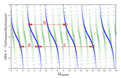
| Fig. 50. Graphical means to solve for the field parameters for Dirichlet boundaries. The ratio of the outer radius b to the inner radius a of the resonator was chosen to equal 3 for this graph. |

|
| Fig. 51. The solutions of (55a) utilizing regions "a", "b" and "c" of the functions as shown. In each solution the wavenumber k would be adjusted using (57) so that the left point of that region would coincide with the inner radius and the right point would coincide with the outer radius. |
The factor b/a is simply the outer radius of the resonator divided by the inner radius.
Of course the two ratios, ratioa and ratiob , must be the same number to determine (55a) up to a single arbitrary amplitude. To computationally solve for the correct choice of the ratio as well as the needed value of k to satisfy the boundary conditions, we plot the two ratios versus unorm in the Fig. 50 at the right: ratioa in blue and ratiob in green circles.
For the sake of definiteness, we set b/a = 3 in this graph. We look for places on the graph where the two ratios equal each other realizing that there will be spurious crossings. The useful crossings are circled in red. The interval labeled "a" represents a valid solution, where the left most end is the point at which the two ratios are equal. The right most end of "a" is a point where unorm is the required 3 times larger than unorm at the left end. Intervals "b" and "c" are similarly valid. Intervals "a", "b" and "c" represent solutions having one half cycle, one cycle, and one and a half cycles of field undulations in the radial direction. We would label these three modes has having indices n = 1, 2 and 3 respectively.
From Fig. 50, intervals "a" and "c" have a ratio A/B = − 0.9 . This fixes the field strengths, up to an arbitrary overall amplitude. The radial wavenumber k is determined by (57) where unorm is read off the horizontal axis of the graph at the left end of an interval. For example, for interval "a" , unorm = 1.6 . The resonator's inner radius a is presumably known so we can solve (57) for k.
One might remember that the index m is set by the number of wave cycles in the φ direction for the particular mode of interest. This azimuthal index m also sets the order number of Jm and Ym. The frequency of a particular mode is set by (53b) above.
Neumann boundaries for annulus resonators
The solution of the fields for annular resonators with Neumann boundaries is basically the same as that above for Dirichlet boundaries with a few changes. We would differentiate (55a) to get:
 , (59)
where J' is defined as
 so that
 . Y' is similarly defined.
In order that dR(r)/dr be zero at r = a and r = b, the terms inside the brackets of (59) must be zero at those points. Just as we did for (56) above, we can define "ratioa" and "ratiob" and end up with equations just like (58) except that derivatives of the Bessel functions replace the Bessel functions. Furthermore, we can graph the two ratios versus unorm and end up with a graph like Fig. 50 which can be similarly interpreted to yield solutions as in Fig. 51.
Added thoughts concerning annulus resonators
Donut shaped resonators can also be considered a form of ring resonators, although often that term implies no radial dependence of the fields inside the resonator, i.e. an n = 0 mode with m > 0. These modes only exist with Neumann boundaries.
Also, rotating modes do exist in donut shaped resonators, the same as they do for the circular resonators covered in Sections 1 through 8 above. A third point: you can combine the pie and donut shapes to have a donut with only part of the full circle there. We merge the solutions for each. We leave it to the reader to flush out the details.
| ⇑ Fig. 52. Animation of radiating wave, m = 0. Mouse over the image to see the action, mouse off to suspend it and click on it to restart it. | ⇑ Fig. 53. Fig. 52. Animation of radiating wave, m = 2. The frequency and radial wavenumber is also different than those in Fig. 52. |
| ⇑ Fig. 54a. Animation of spiral wave, m = 1 (one spiral arm of each color). |
| ⇑ Fig. 55b. Animation of radiating wave, m = −3 (3 arms of each color and rotating in the negative φ direction). |
10. Related radiating waves
Bessel function solutions can also be used for two dimensional waves radiating from a small emitting source. The appropriate wave to use for waves of fixed azimuthal shape is:
 . (60)
These waves are shown in flash animations in Figs. 52 and 53 for two different radiating modes, i.e. different integer values for m and different wave numbers k. The frequency is related to the wavenumber via ω = vp k.
Spiral radiation modes:
The equivalent to rotating resonant modes are spiral radiation modes. Expressed in real sinusoids these are given by:
 , (61)
or in terms of complex notation:
 . (62)

|
| ↟ Fig. 55. Old image of author making spiral waves on water's surface with a stick. |
Animations for spiral radiation modes are shown in Figs. 54a and 54b. There is a nice YouTube video showing spirally gravity waves here.
Use of Bessel functions of the second kind:
Equations (60), (61) and (62) use Bessel functions of the second kind, i.e. Ym(kr) for two reasons. First, in a radiation case, the space of interest does not include the origin. Two dimensional radiation fields have amplitudes that fall off inversely as the square root of the radius. If the fields were extended back to the origin they would be infinite at the origin. Furthermore in real radiating systems, the radiation source occupies a certain space and excludes the origin from the wave field.

|
| Fig. 56. Jm(u) and Ym(u) plotted together versus u. In this graph m = 2 was chosen as typical of these functions. We can see that Ym(u) peaks at the zero crossing of Jm(u) and Jm(u) peaks at the zero crossing of Ym(u). In this sense they are like the sine and cosine functions. |
A second phase provided by Ym(kr)
The second reason for including Bessel functions of the second kind is that they provide a second phase in the r direction, complementing the phase of Jm(kr). We can see this in Fig. 56 where we have plotted Jm(kr) and Ym(kr) together to emphasize their relative spatial phase (phase in the r direction). Having the two phases is required for traveling wave motion in the r direction. Remember in Cartesian coordinates, we use both sine and cosine functions together (or their equivalent) in order to get both spatial phases as required to create traveling waves . This role of providing a second phase is further demonstrated in the animation in Fig. 57 below where the presence of Ym(kr) provides for smooth outward motion of the wave crests and troughs in the bottom graph. For the functions as shown in Fig. 57 the order m equals 2.
| ⇐ Fig. 57. Animation showing the two phases provided by the Jm(u) and Ym(u) functions acting together to make a radiating wave. Mouse over the image to activate it, off to suspend it and click to restart it. In the upper section the function Jm(u) as modulated by cos ωt is shown in blue while Ym(u) as modulated by sin ωt is shown in green.
The lower section shows the sum of the two functions in the upper section. This lower trace changes color depending on whether it is mostly composed of Jm(u) or Ym(u) at a particular time. This variation in composition is caused by the out-of-phase action of the modulating functions cos ωt and sin ωt. The functions are not shown near the origin because Ym(u) become very large there. |
Use of large argument approximations for Jm(kr) and Ym(kr):
We can see the complementary phases as they relate to sine and cosine functions by looking at (60) in the case of very large radii. In this case we can use large argument approximations for Jm(kr) and Ym(kr):
 and
and
 , (63)
to get:

 , (64)
where u = kr and we have used Euler's formula. We can clearly see the traveling wave signature of (kr − ωt) in the argument of the exponent in the final equation.
We can see the dual role of the two phases via sine and cosine terms if we further expand the complex exponential factor:

 . (65)
Modulus and Phase of Bessel functions:
One can get further insight into the phase relationship of Jm(kr) and Ym(kr) with what is known as the modulus and phase of Bessel functions. Also see Abramowitz and Stegun section 9.2.17 page 365.
For this, one considers Jm(kr) to be the real part of a complex function, the Hankel function of the first kind, and Ym(kr) to be the imaginary part of it. Basically:
 . (66)
Note that we used the right side of (66) in Equations (60) and (62) above. The modulus, Mm(u), is the magnitude of this function, i.e.
 , (67)
and the "phase" is the complex argument of the Hankel function:
 , (68)

|
| Fig. 60. Graphs of the modulus and phase of the Bessel function m = 2. The modulus is plotted along with a compensated version of it, i.e. compensated by multiplying it by the square root of u to compensate for the modulus' falling off as the inverse of the square root of u for large values of u. The phase is also plotted. We also plot a version of the phase that has been divided by u to compensate for its tendency to increase linearly with u. |
where atan2(y,x) is an expanded arctan function which returns values over all four quadrants instead the the usual two quadrants.
We have plotted the modulus and phase in Fig. 60 in blue and red respectively. We see that the modulus approaches zero at large u whereas the phase approaches an upwardly sloping straight line for large u.
For a two dimensional circular symmetric system as this is, we would expect the amplitude of the waves to weaken as the wave progresses and spreads out. Since the energy in the wavefront is proportional to the amplitude squared and the width of the wavefront (the circumference), conservation of energy would say amp2×2πr = constant which can be solved for the amplitude as amp = squareRoot(constant/2πr). That is to say we expect the amplitude to be inversely proportional to the square root of the radius, i.e. to 1/r0.5. Furthermore if the phase is like that of a conventional sinusoidal wave whose phase at any one time increases as kx, at any one time our Bessel wave should have a phase that is proportional to the distance, i.e. to r.
In our plot in Fig. 60 we have multiplied the amplitude (the modulus) by the square root of the normalized radius to compensate for the expected proportionality to the inverse of the square root of the radius. We have also divided the phase by the normalized radius to compensate for its expected linear dependence on u. So if the Bessel waves behave as sinusoidal waves do with the added spreading out feature, we would expect our graph to show constant compensated amplitude and phase. We see from the graph (the green and turquoise traces) that we indeed get this behavior at large radii, but not at small radii. The large distance behavior is consistent with our earlier observation that at large distances the Bessel functions can be approximated as sinusoids and behave like sinusoidal waves with the added spreading out feature.
At small radii near their source, Bessel waves are different from sinusoidal waves. We classify this small radius behavior as near field behavior. From the graph we see that it occurs when the normalized radius u = kr=2πr/λ is near one or less. Rearranging we see near field behavior occurs when r < ≈ λ/2π .
11. Modified Bessel functions Im(u) and Km(u) and evanescent waves.

|
| Fig. 61. Graphs of the modified Bessel functions Im(u) and Km(u) for m = 2. |
When the above Bessel functions have an imaginary argument they are called modified Bessel functions and lose their oscillatory behavior. These are solutions to Bessel's equation (43c) when the 1 in that equation becomes −1 [Abramowitz and Stegun, Handbook of Mathematical Functions, p.374, paragraph 9.6.1]. These functions are graphed in Fig. 61. One can see they are similar to the exponential functions e±u . The mathematical definition of these is:
 and
and
 . (69)
When m is an integer, we are to use the limit as m approaches that integer. Also I−m(x) = (−1)m Im(x) and K−m(x) = (−1)m Km(x) .
These functions are solutions of the wave equation in cylindrical situations where waves cannot freely travel and only are able to leak into the region. A good example of this is the field outside the inner core of an optical fiber . These frustrated waves are called evanescent waves.

|
| Fig. 62. Setup for evanescent waves in two dimensions. The inner area, region 1, is a dense membrane (thicker or loaded with an array of weights) while the outer area, region 2, is a light weight membrane. Region 1 has a radius r = a and region 2 has a radius r = b. |
Concrete example of evanescent waves
A good example of evanescent waves occurs on a diaphragm similar to that shown in Fig. 48a but modified to use two different weights (per area) of diaphragm material: an inner heavy material, material 1, and an outer lightweight material, material 2, as shown in Fig. 62. In this system evanescent waves occur in the outer region (region 2) when we excite a whispering gallery mode in the inner region, i.e. a mode that has a large m index and n = 1.
We choose for the fields for the two regions to be:
 , (70a)
in the inner region where r < a and:
 , (70b)
in the outer region where a < r < b. In these equations we have arbitrarily set the amplitude of the wave in region 1 to be one and also assumed that the wavenumber in region 2 is α times that in region 1. The constant α is proportional to the square root of the mass densities of the two membrane materials. We assume α << 1. We also assume that all the waves are standing waves and therefore all are in phase.
At the junction (interface) between the materials we have the two conditions:
- The vertical displacements of the membranes due to the waves on either side of the interface must be equal: ψ1 = ψ2 at r = a.
- In order that the wave induced vertical forces be equal on both sides of the interface, the r derivatives of ψ on both sides must be equal, i.e. dψ1/dr = dψ2/dr at r = a.
Written more formally these conditions are:
 (71a)
(71a)
and
 . (71b)
With Dirichlet boundaries, the waves at r = b should equal zero:
 . (72)
The above equations (71a), (71b) and (72), can be simplified as:
 (73)
(73)
 (74)
(74)
 . (75)
We have three equations, (73), (74) and (75) and three unknowns, A, B and k. So in theory we should be able to solve for the unknowns. We solve the last equation for A and substitute the result into (74) to yield:
 (76)
(76)
 (77)
(77)
 . (78)

|

|
| ⇑ Fig. 63. Plot of the two sides of (73) with m = 10 and α = 0.3 . We see the solution to (73) is k = 13.3 . This is the point where the two curves cross, so the left hand side equals the right hand side of Equation (73). | ⇑ Fig. 64. Plot of (70a) and (70b), i.e. of the fields in the regions of two different radial wavenumbers showing evanescent wave behavior. The fields in region 2 do not have the space to complete even one half oscillation in the radial direction and so mimic exponential behavior. The parameters used were the same as in Fig. 62. |
| More on Fig. 64:
The two terms in (70b) are plotted separately to show the size of each. The red curve is slightly offset to avoid covering up the blue curve and to show that it coincides with the blue curve in region 2. The AJm(αkr) term (green) is essentially zero over the region of interest (region 2) while the BYm(αkr) term (in red) dominates and coincides with the total fields (blue) in region 2. | |
We next proceed with the rest of the solution numerically. We choose m = 10, a = 1, b = 2 and α = 0.3 .
Equations (76) and (78) are both functions of the wavenumber k. In Octave we use (78) and (76) to calculate the left and right hand sides of (73) for a series of k values. We have plotted the two sides versus k in Fig. 63. We look for points on the graph where the two sides are equal. We see the equality point, i.e. the solution, to (73) is at k = 13.3 . The constants A and B for this k value are B = −0.00102 from (78) and A = −0.0165 from (76).
In Fig. 64 we show a graph of ψ versus r using these values. In Fig. 65 we show a color plot of the fields versus r and φ using our calculated values of k, A and B in Equations (70a) and (70b) for the two regions. Note that the fields leak into the second region and are pretty much kept absent from the region's edge at r = b.

|

|
| ⇑ Fig. 65. A color plot of the fields we have solved for, showing the radial and φ dependence in false color. The inner region and outer region are shown with circles at r = a and r = b, i.e. radii of 1 and 2. We see that the fields are largely at the interface of the two regions as we might expect for an m = 10 mode. This is a good example of a whispering gallery mode. Also, this mode could be made to rotate by combining it with its twin mode with a quarter cycle phase shift. | ⇑ Fig. 66. Graph comparing J10(u) and Y10(u) with J0(u) (in red). We see that J10(u) (in blue) and Y10(u) (in green) do not start their oscillations until higher values of u whereas J0(u) starts at u = 0. The higher the m value (the order of the Bessel function), the higher the u value for starting the oscillations. |
We might ask the question of how the Bessel functions work to numerically exclude the fields from around the origin. For this example we have picked m = 10. In Fig. 66 we have plotted J10(u) (in blue) and Y10(u) (in green). We see that such a high m value means J10(u) does not start its oscillations until larger values of u = kr occur, excluding Bessel fields from the region around the origin. We might respond that Y10(u) is not zero around the origin, but then again Y10(u) is not to be used around the origin because it becomes infinite there (see Equation (70a) .) Only J10(u) is to be used in region 1 around the origin and J10(u) is effectively zero in this region. The physics of the issue is that at the excitation frequency of the resonance, the distance between adjacent peaks would become very small if the fields were to include the region close to the origin, much smaller that the wavelength at this frequency.
We might note that the above example, while showing evanescent waves, does not utilize the modified Bessel functions Im(kr) and Km(kr). Note also that if we had picked larger k's from Fig. 63, from crossings farther to the right, we would have more peaks in the radial direction. Depending on which crossing we pick, we could have more peaks in region 1 or one or more in region 2.