Reflection of waves as a process to make standing waves

   In memory of author Hans Christian Andersen and sculptor Edward Eriksen and their The Little Mermaid, Copenhagen, Denmark, 1836 and 1913

Waves usually reflect when they hit any sort of obstruction or change in the media. Sometimes the reflection is total, other times it is partial with the non-reflected waves continuing, being absorbed, or partly continuing and partly being absorbed. Above and below we show animations of the reflection process, as demonstrated with waves on a rope above and with water waves below. Mouse over the animations to start them, off to suspend them, or click on them to restart.

No reflection

We will focus mostly on the animation below which is set up to demonstrate a number of different reflecting conditions and principles. This animation initially starts with "no reflection" active. In this setting, we see a pure traveling wave with no reflection. Some of the features of this wave are:

• There is a pure traveling wave, propagating from left to right, unimpeded.
  
  
• The light gray region around the surface of the wave shows the envelope of the wave. This is the region swept by the wave (i.e. the water surface) as the wave passes. You can see that for this pure traveling wave, the envelope is constant, does not vary with x, and that all points are swept equally as the pure traveling wave passes.
  
  
• The envelope's minimum amplitude equals its maximum amplitude, as indicated by the little "min" and "max" bubbles. This equality is always true for a pure traveling wave with no attenuation.
  
  
• Below the wave, we see the phasors, for various points along the wave. Note that where the wave is maximum, at the wave crests, the phasors are pointing to the right, totally on the real axis, in which direction the real part is maximum. The phasors at the wave troughs are pointing in the opposite direction, to the left, where the real part is negative.
  
  
• The phasors are all of the same length and point at progressively different angles. This is always true for a pure traveling wave (having no attenuation).
  
  
• Along the bottom edge, a little right of center, we see a number for the standing wave ratio. The standing wave ratio is a measure of the amount of standing waves in the system. It is defined as the envelope's maximum amplitude divided by the envelope's minimum amplitude, as indicated by the max and min bubbles. In this case of zero reflection, it equals one since the min equals the max. This value of one is indicated for the standing wave ratio at the bottom edge of the animation. A standing wave ratio of 1 means no standing waves are present, that the waves are purely of the traveling wave type. We will discuss the standing wave ratio more below.
  
  
• The notation in the center of the bottom edge of the animation indicates that the reflection coefficient is zero, meaning that there is no reflection in this case. The angle of the reflection coefficient is indeterminate since there is no reflection. This is indicated by a question mark.

Click here for a copy of the above animation in a separate window that can be sized (even to fill the entire screen) and positioned independently from the text. Your popup blocker may prevent a separate animation from being launched. In some browsers the separate animation will stay on top if you only use your scroll wheel to scroll down this text, and do not click on the text.

Click here for a slightly different version of a separate window. This version allows you to save the animation to a file by clicking on "file" and then "save page as" to get this animation into your computer. Please read the fair use policy.

Total Reflection, no phase shift

If you click "total reflection +", you see a sea cliff appear on the right hand side which will reflect 100% of the waves.

• Wait for the wave to propagate up to the cliff, reflect, and travel back across the screen. At this time you will see the formation of a pure standing wave formed by the 100% reflection of the incident wave. As we saw in the last two postings, a standing wave is the superposition of two equal, but oppositely propagating traveling waves, which is exactly the situation in this case where we have 100% reflection.... all of the incident wave is reflected giving an oppositely propagating traveling wave in addition to the incident wave.
  
  
• In this case, you see that the light gray envelope of the pure standing wave is not constant as it was with the no reflection case, but has well defined peaks called antinodes or maximums, and minimums called nodes or zeroes.
  
  
• The minimums of the envelope of a pure standing wave are zero, i.e. the wave has zero amplitude at the minimums, which is again different from the no reflections case. At these points, there is no vertical motion of the water surface, even though the wave field is very active on either side othe these points.
  
  
• A maximum occurs at the reflecting surface.
  
  
• The standing wave ratio (the max divided by the min) is now equal to infinity, since the denominator, the minimum, is zero.
  
  
• The reflection coefficient is now 1.0 or 100%, and the phase angle of the reflected wave is 0°. This means that the phase of the wave immediately after reflection equals that of the wave immediately before reflection.
  
  
• The phasor pointers, while still rotating, are pointing all in the same direction or at 180° from the rest. Their lengths vary in proportion to the amplitude of the envelope at a particular point. This is quite different from the case of the pure traveling wave we looked at first, where all phasors had the same length but different directions.

Total reflection, 180° phase shift

If we click on "total reflection −" we have a setup where the wave undergoes a 180° phase shift upon reflection.

• Such a phase shift is rather hard to achieve for water waves, but it is a common occurence in some wave systems such as in the case of a sound wave traveling down a tube...an open end of the tube will cause a near-perfect refection with a 180° phase shift. It is also the most common reflection for waves on a string or rope, such as in the mermaid animation at the very start of this posting. Hold the mouse button down on that animation to achieve longer wave trains to more clearly see the standing waves.
  
  
• The envelope, or light gray region, is very similar in shape to what it was with "total reflection +" case, only that the maximums and zeroes are shifted over from before. Now, a zero or node occurs at the point of reflection. We get a zero because the reflecting object causes a 180° phase shift in the wave, so that the reflected wave is 180° out of phase with the incident wave right at the point of reflection and the two waves cancel there.
  
  
• The complicated reflecting barrier shown (in the second animation), as is needed to cause such a phase shift in water, will not have a single flat reflecting surface, but we will consider the effective "reflecting surface" to be at the right hand edge of the animation. A minimum, i.e. zero, occurs at this "reflecting surface".
  
  
• As before, the standing wave ratio is infinite because the minimum is zero giving a zero in the denominator.
  
  
• The reflection coefficient listed on the bottom of the animation is 1.0 with a phase angle of 180°.

Variable refection coefficient

If we click "variable reflection" the animation uses a random number generator to set, at random, the reflection coefficient and the phase angle. If you don't like the values selected, click on it again for a new set of values.

• The reflection coefficient and phase angle selected are shown in the center of the bottom edge of the animation.
  
  
• The envelope will now be somewhere between the three cases above, with minimums and maximums, and where the minimums are not zero.
  
  
• The standing wave ratio (the maximum divided by the minimum) will be some number larger than 1.0 but smaller than infinity. This means we have something between a pure traveling wave and a pure standing wave. We can think of this as a mix of the two: perhaps a standing wave with a extra traveling wave added to it.
  
  
• The phasor pointers vary in length and in the direction they point.
  
  
• These waves are fascinating to watch. The wave field has a traveling wave component that continually travels to the right. At the same time the waves have these envelope minimums to slip through. No matter how tight the minimums are, the waves somehow manage to configure themselves to magically slide through the constrictions.
  
  
• We can click "show components" to see a mathematical dissection of the wave into two pure traveling waves. The red part is a traveling wave propagating to the right and the blue part is a traveling wave propagating to the left. The amplitude of the blue wave will be less than that of the red wave, since only a fraction of the red wave is reflected (the ratio of the two equaling the reflection coefficient.) You can watch how the two wave components slide in opposite directions, making the maximums in the black total wave when their peaks pass each other.
  
  
• I have shown as a reflecting barrier, a messy, wave absorbing, seaweed choked cliff with under seas rocks, as might be expected to produce a reflection coefficient with a partial reflection and complicated phase angle.

Math of reflections

We can mathematically express the "incident" wave, as:

,

where we have shown both the cosine and the imaginary representations.

The "reflected" wave is just this incident wave times the reflection coefficient and shifted in phase by the phase of the reflection coefficient. We also need to change the sign of the wavenumber κ because the reflected wave is traveling in the reverse direction from the incident wave. In addition, it is important just where the reflection takes place. For the moment, we will assume that it takes place at x = 0, placing the x origin on the far right side of the screen and all the wave activity is in the negative x region. The equation for the reflected wave is:

,

where Γ, capital gamma, is the complex reflection coefficient and is defined as Γ=re^iφ where r is the magnitude of the reflection coefficient, is real and is defined as the amplitude of the reflected wave divided by the amplitude of the incident wave. As is typical of the complex form of phasors, both the magnitude and the phase of the reflection can be characterized by one compact complex constant, Γ. The complex reflection coefficient is defined as the complex reflected wave divided by the complex incident wave, both evaluated at the point of reflection (x=0 in our case). The phase shift φ is the phase of the reflected wave just after reflection minus the phase of the incident wave just before reflection (both at x=0 for our case).

We can easily check out if the above equation for the reflected wave is consistent with our description in the text. To do this evaluate the equation for the incident wave at x=0 to get:

.

The above equation for the reflected wave at x=0 gives:

.

So you see that indeed, the reflected wave equation is just the incident wave multiplied in amplitude by r and shifted in phase by φ.

Another note: there are two standard variations of the lower case phi and internet browsers are very inconsistent on which variation they use. Rest assured that         and          are the same greek letter and stand for the same mathematical quantity. The phi's occurring in equations that are entered as bit maps may be of other variation from those that have been entered as html code, depending on your browser.

The total wave field

• The total wave field consists of the sum of the two waves discussed above. Thus we sum the incident wave and the reflected wave:

  ,

  as written in the cosine notation.

• The same wave field written in the complex notation is:

  

  .     (1)

  This last equation sees extensive use in the design of electronic communication devices that use waves to transmit information.

Special cases, total reflection

• In the special case of positive total reflection, where φ=0 and r=1, then Γ=1 and the last equation becomes

  .

  This is the same as derived in the previous posting for a standing wave.

• In the case of negative total reflection, r=1 as before, but φ=180°. This makes Γ = re^iφ = -1, making our equation become:

  .

  This is similar to the above equation for the φ=0 case, however it is shifted both in position (by π/2κ) and in phase (by i = e^iπ/2 or 90°). We see this shift in the animation if we compare the standing wave pattern of the "total reflection+" case with that of the "total reflection −" case.

In the above we have used the following relationships, which are easily derivable from Euler's formula (just substitute Euler's formula in for the e^iα and e^−iα to verify these):

 (1a)

.

The standing wave ratio

The standing wave ratio is defined as the maximum amplitude in the wave field divided by the minimum amplitude:

.     (2)

This can be expressed in terms of the reflection coefficient by realizing that the maximum of the amplitude occurs where the incident and reflected waves are in phase. Look at the phasor dials in the animation above to see this (with "show components" and "total reflection" active). Similarly, the minimum occurs where the two are out of phase. When in phase they add up to an amplitude of A+rA and when out of phase they add to A−rA. Thus we can write the reflection coefficient as:

.

This equation is graphed to the right. We can also use this to solve for the reflection coefficient r in terms of the standing wave ratio s to give:

.     (3)

Position of the envelope maxima

We can also use these concepts to calculate the position at which the maximums and minimums will occur. If we are a distance  l  from the reflection, then the phase shift for the incident wave to travel up to the reflection is κl . There it undergoes a phase shift of φ upon reflection and then an additional phase shift of κl returning to our spot as the reflected wave. Thus the phase difference between the incident and reflected waves at this spot is 2κl+φ. To make a maximum, this phase difference must be an integer multiple of 2π radians. Putting this into an equation gives:

,    (4)

where n is an integer and represents the number of the particular maximum we are considering. The first maximum from the reflecting object (just to the left of the object) would have an n = 1, the second one from the object has n = 2, and so on. The wavenumber κ can be calculated from the wavelength λ (the distance between wave crests of the incident wave) as:

κ = 2π/λ.     (5)

We can solve Equation (4) for the necessary distance l for an envelope maximum to occur:

.

where φ is the phase of the reflection coefficient. Alternately, we can solve for the phase of the reflection coefficient in terms of  l:

.    (6)

The most common utility of the standing wave ratio is that it allows determination of the reflection coefficient, angle and magnitude, from simple measurements on the wave field. Observing the waves, one can obtain the wavelength λ and from that the wavenumber from the Equation (5) above. One can also measure the wave amplitudes at the maximum and minimum and calculate their ratio, or s (Equation (2) above). Using the Equation (3) above this gives the magnitude of the reflection coefficient r. Measuring the distance l from the reflecting obstacle to the first maximum and using the Equation (6) above with n=1, gives the angle of the reflection coefficient.

Location of the envelope minima

If one wishes instead to measure the distance to the minimum, then we need to alter the relationship Equation (4). In this case, we need the phase length to be some odd integer of π radians or 180° so that the incident and reflected waves will be 180° out of phase and try to cancel. So setting the phase shift due to the distance and reflection ((2κl+φ) to the odd integer of π gives:

,

where m is an odd integer (n=1, 3, 5, or 7, etc.). This can be solved to yield:

and

.

This brings us to an interesting point. The phase angle of the reflection coefficient depends critically on the location we select as the reflecting point. In some situations, this reflecting point is clear, as it was with our "total reflection+" case where there was a sheer cliff. However, often there is not an exact point that reflects the waves, such as in the "total reflection-" or "variable refl" cases. Then, in the interest of maintaining simplicity, one chooses an "effective" reflection point. With regard to the above animation, we chose the right edge of the animation, for simplicity, and calculated a set of reflection angles based on this. If we had chosen another effective reflecting point, then we would have calculated another set of reflection coefficient angles for the same total wave fields, in order to account to the different phase lengths involved with a different idealized reflection point.

Equation for the envelope

To get an equation for the envelope or magnitude of the total wave field as a function of x, we revisit Equation (1) above. One approach is to use a carefully drawn phasor diagram of Eq. (1) and the law of cosines to arrive at an expression for the magnitude of the wave field. We shall do that first. Another approach is to simply separate out the real and imaginary parts of (1), square each, take the square root, and simplify a bunch to find the magnitude. We do that secondly, below.

We do the vector sum of phasors as follows:

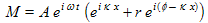
• To the right, we have drawn a phasor diagram (in the complex plane) showing the vector addition of the left side of Eq. (1) with the A e^iωt factored out, i.e.     
  
  
• There we see red vector representing e^iκx  is of length 1 and is drawn at an angle of κx with respect to the real axis.
  
  
• The blue vector represents  reⁱ(φ-κx)  and is of length r and angle (φ−κx).
  
  
• The angle B between the red and blue vectors is given by B = (φ−κx)−κx = φ−2κx.
  
  
• The angle C equals angle B (and therefore also equals φ−2κx ), because their two sides are parallel.
  
  
• The supplement to C, angle D, is given by D = π−C = π − (φ−2κx), where π radians equals 180°.
  
  
• By the law of cosines, the magnitude M is given by:
       .
  
  
• We can simplify the cosine:
       .
  
  
• This allows the magnitude to be written as:
       .
  
  
• Putting in the amplitude A that we left out, gives us the amplitude (half the thickness of the envelope) as a function of position:
       .

  Note that A is the amplitude of the incident wave by itself.

An alternative way to derive the above expression that doesn't involve drawings of vectors is as follows:

• We start with the same complex phasor expression of incident and reflected wave, Equation (1), but we factor out half of the reflection angle as:

  .
  .
  
  

• The first factor is simply a magnitude times the complex temporal rotor times a constant phase shift. We ignore this for now and focus on the rest, which we will call M₁.   M₁ is similar to the expression for the cosine (Equation (1b) above), except for that factor of r. To get around the r, we peel off an r amount of the first term and combine it with the second term to make a cosine. Also, we still have the rest of the first term, which we put first:

  
  .
  
  

• The cosine term is totally real, so only has a real term, and the other term has both a real and an imaginary term, via Euler's formula. To take the magnitude of M₁, we use the square root of the sum of the squares of the real and the imaginary parts. So under the square root, we need to add the two real terms and square their sum, and to that add the square of the imaginary term.
  .
  
  
• We expand and combine terms and finally use the identity sin²x+cos²x=1:
  .
  .
  .
  
  
• Using the double angle formula for cosine, we get:
  .
  
  
• Symmetry of the cosine, i.e. cos(−x)=cos(x) allows us to write it as:
  .
  
  
• This is the same expression as we got above.

Practical applications of reflection concepts The concepts discussed above are of great use in modern communication systems, where electromagnetic waves carry information. These waves may be in air, in space, in a cable, or in an optical fiber. In most cases engineers seek to minimize reflection, so that the waves are almost completely absorbed by a receiver, where they are most needed and will not reflect and cause spurious ghosts or extra noise in the system. Engineers use these equations to design receivers and other components to minimize reflections and optimize other performance features. The commonly used Smith Chart is a graphical method to approach reflection problems and is based on the above equations. A biography of the inventor, Mr. Phillip Smith, is here and a very short history is here.

The animations in this posting can be downloaded free from George Mason University Archival Repository. Please read the fair use policy for this work.
© P. Ceperley, 2008.

---

NEXT: Water waves PREVIOUS TOPIC: Complex phasor representation of a standing wave

---

Good references on WAVES

Good general references on resonators, waves, and fields

Wikipedia on waves. Zona Land on waves, lots of animations. The physics classroom on waves. Thinkquest on waves. Dr. Dan Russell, Kettering University Applied Physics, nice animations. All sorts of demonstration setups and animations from the Univ. of California at Berkeley. And many more sites.... search on waves and traveling waves. Scroll down farther for a list of the various related topics covered in postings on this blog.

Think Quest -- Wave Express technorati.com The Physics Classroom HyperPhysics intutor.com Wikepedia

Complex phasor representation of a standing wave

Standing waves and resonances are at the heart of musical instruments, electronic technology, and atomic systems. In this posting we examine standing waves in another dimension, adding the complex dimension. In the last posting, we introduced standing waves. We examined the phasors for standing waves at isolated points along the wave. We can extend this to a continuous representation of the phasors, similar to what we did for traveling waves in the posting on Waves using complex phasors.

The animation below as it initially starts, shows a single traveling wave in a rope in front of a gridded wall. We are assuming that there is no reflection of waves at the far end, in all aspects of this animation. Mouse over the animation to start it, and mouse off to suspend it, and back on again to allow it to continue. This is useful if you want to examine it stopped. You can click on the animation to cause the waves to be restarted from zero. If you click on "right", a traveling wave will be launched from the right. The "both" button will give you two traveling waves, traveling in opposite directions. Once they meet and interfere, you will see a standing wave as discussed in the last posting Superposition and standing waves.

The man and woman are holding on to either ends of the rope. Waves on the rope are the only "real" waves in this animation. The rest of the "waves", that you are about to examine, are waves in the phasors, which in turn are just a way of keeping track of waves, but are not real, physical waves themselves...just like a clock face is not the time, but it shows a representation of the time. On the other hand, even though waves in phasors are not physical waves, understanding them is central to the understanding of waves.

If you turn on (click on) "both" and "components", you will see the two traveling waves that make up a standing wave. As before, you can observe the two traveling waves sliding in opposite directions to cause (or add up to) the standing wave. As before, the appearance of the two traveling waves is quite different than the standing wave. The traveling waves maintain their shapes as they slide along, while the standing wave does not move, but oscillates in place. I should state again, that only the wave on the gray rope is real or physical. The pink and bluish "waves" show what you would observe if you had only one of the traveling waves. The two waves represent the mathematical dissection of the standing wave.

Click "components" again to turn off that feature for a minute. Now click on "phasors". This will show you a continuous helical representation of the complex phasor of the wave, similar to that seen in Waves using complex phasors. I show phasor diagrams every so often on the x axis. In principle there should be a phasor diagram for every possible point on the x axis, but that would obscure the phasor waves. Alternately, I could have not shown the phasor diagrams and said the phasor wave is plotted in a special "space", where one axis is imaginary displacement of the wave, one is the real displacement of the wave, and one is the propagation direction. To see such a plot of the phasor wave in this special space, click on "phasor dials" to hide the phasor diagrams.

When the animation starts afresh, (click on it to restart it if needed) and if the "left" or the "right" button is activated, a helical phasor wave will be launched from the appropriate end. This phasor wave represents the loci of all the tips of the phasor vectors in the phasor diagrams for varying x and time. When "both" is active, helical phasor waves are launched from both ends and come together in the center to interfere. What results is quite unintuitive. It is not at all a helix. Instead, the resulting phasor wave lies entirely in a plane, a plane that rotates about the axis of propagation. It looks like the standing wave at its maximum (see the standing wave to the left of the phasor) but now instead of oscillating in place, the complex phasor wave spins around the x axis. The phasor looks a bit like a potato masher twisting along its axis. This illustrates on of the important features of a standing wave, that the phase is the same (or 180° different, equivalent to a minus amplitude) at all point along it. This phase changes in time, but it is not a function of position, as it is with a traveling wave.

If you read the labeling on the phasor diagram axes carefully, you will see that we have twisted the axes of the complex plane by 90° from the normal orientation; so that the real axis is vertical. In this orientation, the actual standing wave is the projection of the phasor wave, projected to the left. That is to say, the actual wave is like a shadow of the phasor if the light were coming in horizontally and casting the shadow of the phasor onto the vertical tiled surface.

You can now turn on the "components". The result is somewhat complicated .... quite a tangle so don't be too disappointed if you have trouble following my explanation. If you skipped some of the discussion above, you might want to revisit it. You need to understand that before working on the full complexity of phasors with the components showing. It also might be useful to mouse off the animation from time to time to stop it and examine all the details better. The animation shows the red and blue helical phasor waves for the two traveling waves, in addition to their sum, the standing wave. Note that there are red and blue vectors on the phasor diagrams (the "phasor dial" need to be on to see this). If you study the animation carefully in this setting, you will see that the phasor wave of one component is a helix traveling in one direction, and that of the other traveling wave is a helix traveling in the other direction. At any particular plane, for example, at one of the planes of the phasor diagrams, the three waves are represented by vectors, all of which are rotating in the same direction (counterclockwise) and at the same rotational speed. At different phasor diagrams, the angle between the red and blue vectors differ and consequently their sum varies.

You may have noticed that the wave motion slows down when the "phasor" button is activated and that the "components" slow it down even more. These additional features increase the amount of computations that your computer is doing and can result in a slower animation. A faster computer will slow down less.

The math of complex helical phasors for standing waves

In the previous posting Superposition and standing waves, we derived equations for the cosine representation of a standing wave:

.

The complex representation of the same wave was derived to be:

.

We see that in the cosine representation, the x function, cos κx, is multiplied by the time oscillating function, cos ωt, producing an oscillating version of the original x function. This is what we see in the animation above for the actual wave, the one on the left against the gridded wall. On the other hand, in the complex representation, the space function cos κx is multiplied by the complex rotor function e^iωt. The complex rotor function has a constant magnitude of one and rotates in time in the complex plane as seen in a previous animation on Complex phasors. It is this complex rotor that is responsible for spinning the phasor in the complex plane. Thus in the complex representation, we see a constant space function rotating in the complex plane as shown in the animation above.

As is always the case, the actual wave is the real part of the complex phasor. So it makes sense that the actual wave is the horizontal projection of the complex phasor wave, remembering that our real axis is vertical.

Physical helical waves on a rope

One additional point, that I might clear up is that you can easily make an actual or physical helical wave on a rope, and also that a superposition of two such waves propagating in opposite directions looks just like the phasor wave in the animation above. You might get a rope and a friend and try this. At the same time, such a helical wave is not exactly the same thing as what we are trying to portray in the animation above. In the animation, the rightmost wave is the complex phasor wave representing the actual flat standing wave to the left. One of its axes is imaginary. The helical wave in the animation is solely a mathematical representation of a real planar wave on a rope. The complete complex phasor representation of an actual helical wave on a rope would require five dimensions and thus is very hard to illustrate. Most scientists and engineers simply write the complex formula for the phasor of this wave and stop there. If they really want a picture or animation, they would draw a complex phasor drawing for each component of the wave, that is, two complex phasor wave drawings. We'll stop here, since this is probably a little too much complication for this level. Even though these complex phasors can be difficult to draw, animate, or visualize, wave related calculations are made much easier by their use.

The animations in this posting can be downloaded free from George Mason University Archival Repository. Please read the fair use policy for this work.
© P. Ceperley, 2008.

---

NEXT: Reflection of waves as a process to make standing waves PREVIOUS TOPIC: Superposition and standing waves

---

Good references on WAVES

Good general references on resonators, waves, and fields

Wikipedia on waves. Zona Land on waves, lots of animations. The physics classroom on waves. Thinkquest on waves. Dr. Dan Russell, Kettering University Applied Physics, nice animations. All sorts of demonstration setups and animations from the Univ. of California at Berkeley. And many more sites.... search on waves and traveling waves. Scroll down farther for a list of the various related topics covered in postings on this blog.

Think Quest -- Wave Express technorati.com The Physics Classroom HyperPhysics intutor.com Wikepedia

Superposition and standing waves

The animation below shows two types of waves: transverse waves on a rope and longitudinal compression (i.e. very slow acoustical) waves propagating through a line of squishy balls full of water. The compression waves are made clearer by having the color of each ball change in response to the compression of the ball, to red as a ball is compressed and to blue as it is stretched. To see the animation, mouse over it. To stop it, mouse off it. To restart it, click on it.

As the animation first opens (with only the pulse option clicked on... having a red square), it shows two short bursts of traveling waves being launched from the two ends of each wave system. At first, these bursts separately travel towards each other. At some point, they overlap and cause a complicated interference pattern. Then once they are through each other, they resume their simple sinusoidal shape and travel to the end where they are absorbed. During the interference time, we see a brief glimpse of the standing waves we will be discussing below.

If we click on "phasors" we see a phasor diagram in each of the balls, showing the "state of the wave" at each point along the medium. Just to remind you, a phasor is a vectorial diagram showing the amplitude and phase of a sinusoidal wave at a particular point. The phasor in a particular ball is correct, both for the longitudinal wave going through that ball and for the transverse wave in the rope directly above the ball. The phasor diagrams normally would be drawn so they are stationary, but we took artistic liberties on this, having them move back and forth with each ball. They also compress and stretch with the balls.

We can use the animation to understand the phasors and the waves they represent in three regions:

• In the non-interfering part of the wave, i.e. inside the pure traveling wave part, we see that the amplitudes (magnitude or length of the vectors) are constant, while the phases (the angles of the phasors) are continually changing, i.e. the phasors constantly rotate in a counter-clockwise direction.
• Where there is no wave, the magnitudes are zero. The angles, i.e. phases, are indeterminate since the vectors have zero lengths.
• In the interference zone, the phasors have different magnitudes at the different points and they also still rotate.

If we click "components" we now see extra red and blue ropes once the waves are launched. Note that in the sections with no waves, all three colored ropes are bunched together and hard to distinguish. The red rope shows only the wave launched from the left, while the blue one shows the wave launched from the right. The black rope shows the sum of the two waves. That is, at each point in the horizontal direction, if we sum (for a particular x value) the deflections of the red and blue ropes, we will get the deflection of the black rope. This is the principle of superposition, that in a linear system, such as these, when two waves travel through each other, the response of the medium is just to add the deflections of the two waves at each point. We also see that in the interference region, the phasors now show red and blue vectors in addition to the black one. Note that in each ball, the black vector is the vector sum of the red and blue vectors. Note also that the red phasor is the correct phasor for the red rope's wave, and the blue one is correct for the blue wave. Because the red phasor is in front of the blue one which is in front of the black one, the red tip is made a little smaller than the blue tip which is smaller than the black tip to allow you to see a little of all of them when they are together. At the same time, they are very small and it takes sharp eyes to distinguish them in this case. For example, you will have to look very closely to see the red and blue phasors in the interference region at the very center where all three vectors are aligned.

Animation showing the process of superposition of two traveling waves to make a standing wave

If we click the "continuous" button, a continuous sinusoidal wave will be launched from the two ends (this may take a bit of time to get started). At first, we see two waves traveling towards each other and interfering. In time, the interference zone takes over the whole space. When this happens, we have what is called a standing wave on the black rope. A standing wave results from the superposition of two traveling waves. You can probably see the standing wave best by unclicking the "components", i.e. just click on "components" again to turn off its red indicator.

• A standing wave has a different appearance from a traveling wave.
  • A traveling wave keeps its shape and appears to slide along (focus on just the red wave to see the "sliding" of a pure traveling wave).
  • A standing wave, the black wave, oscillates in place and appears stationary.
• A standing wave has "nodes", places where the wave amplitude is zero, pointed out on the animation above by the stationary black arrows.
• It also has "anti-nodes" half way between the nodes where the wave oscillates at its maximum amplitude.
• This author prefer the terms "zeroes" and "maxima" instead of nodes and anti-nodes.

Looking at the waves on the rope, we can understand the mechanics of the standing wave formation. The red and blue traveling wave, propagate to the right and left, respectively (click again on "components" to see this and focus on the red or blue wave). The zeroes (nodes) are located at points where the red and blue waves are mirror images of each other and cancel, producing zero sums at these locations. We see in the phasors, below the zeroes, that the red and blue vectors (or phasors) are pointing in opposite directions (180° apart) and the black sum vector is zero, and therefore not visible.

The maximums (anti-nodes) occur where the two traveling waves equal each other. When the red wave is maximum, the blue wave is also maximum at these points. It is rather fascinating to center your attention on a maximum and watch the red and blue waves slide in a symmetrical way towards this point from opposite directions. A look at the phasors below these point reveals red and blue vectors pointing in the same direction, which is also the direction of their sum, the black phasor. As pointed out before, when the vectors are aligned it takes a sharp eye to distinguish the individual vectors. At these maximums (anit-nodes), the red and blue waves are "in phase" with each other, have 0° phase difference, and add in a maximal way.

At other points besides the zeroes and maximums, the phase shift is somewhere between 0° and 180°. At these points, you can see all three vectors: the red, blue, and black (sum) ones. Note that the phasors in all the balls rotate counterclockwise. Also note that the black, sum phasors, all are pointing in the same, or in exact opposite, directions at any point in time (mouse off the animation to freeze the motion). On the other hand, the traveling waves (such as the red or blue waves) have phasors that vary in direction along the length of the wave.

Math of standing waves done with cosines

The cosine equations for transverse traveling waves propagating in the positive and negative directions are

    .

The similar equations for the pressure in longitudinal compression (acoustical) waves are

    .

A standing wave is a superposition of two equal traveling waves, propagating in opposite directions and is given by the sum of the two above waves:

.

The above is correct for transverse waves. For the compression wave, the equation is practically the same:

.

By using the cosine equation,

,

we can change these sum formulas into

.

The right most part can be rewritten with emphasize on the relevant terms as

.

Thus we see that the basic x sinusoid, cos κx, is multiplied by the time varying function 2A cos ωt. By the process of adding two shifting, traveling waves together, by interfering them, we no longer have a shifting function f(ωt ± κx), and instead have a stationary cosine whose amplitude cyclically varies with time. This is just what the animation above shows. When we have a fully developed standing wave, the magnitudes or lengths of the phasors vary in proportion to cos κx.

Almost as if by magic, two oppositely moving traveling waves interfere to produce a quite different, standing wave.

Math of standing waves with complex phasors

Complex phasors can be used to simplify the above math. We do that here, repeating the above work using complex notation for the waves.

The sum of the two oppositely moving traveling waves is

.

In contract to cosines, exponentials are easy to factor using

.

Thus our complex superposition equation becomes

.

This can be further reduced with the equation

,

which is easy to derive from Euler's formula. Using this gives

.

Just as in the cosine derivation, we end up with the conclusion that the sinusoid, cos κx, is multiplied by the time varying function 2A exp iωt. Of course there is the implied "real part of" associated with complex phasors. If we take the real part of the last equation, we get:

which is the same as the result in the cosine derivation.

If we hadn't explained all the steps, our derivation would have looked like:

.

The animations in this posting can be downloaded free from George Mason University Archival Repository. Please read the fair use policy for this work.
© P. Ceperley, 2008.

---

NEXT: Complex phasor representation of a standing wave PREVIOUS TOPIC: Types of waves (2D waves, EM waves, longitudinal waves)

---

Good references on WAVES

Good general references on resonators, waves, and fields

Wikipedia on waves. Zona Land on waves, lots of animations. The physics classroom on waves. Thinkquest on waves. Dr. Dan Russell, Kettering University Applied Physics, nice animations. All sorts of demonstration setups and animations from the Univ. of California at Berkeley. And many more sites.... search on waves and traveling waves. Scroll down farther for a list of the various related topics covered in postings on this blog.

Think Quest -- Wave Express technorati.com The Physics Classroom HyperPhysics intutor.com Wikepedia