Relativistic mass

all topics by author

introduction to relativity

contents of mathematics of relativity

previous: transforming velocities

next: relativistic kinetic energy

A small mass requires a small force to get it to accelerate at a certain rate.	A large mass requires a large force to get it to accelerate at the same rate.

A small mass moving at a certain velocity will have a smaller momentum than a large mass moving at the same velocity. In a collision, the object with the smaller mass will undergo a more abrupt change in its velocity.

A large mass moving at the same velocity will have a larger momentum. In a collision, the object with the larger mass will experience less change in its velocity.

10. Relativistic mass

Mass has to do with momentum. Indeed the desire to maintain the principle of momentum conservation in all reference frames led Einstein to decide that mass must vary with velocity (at extremely high speeds).

Incidently, Lorentz's view would be that the mass of a particle would actually increase at very high speeds (relative to "the" absolute reference frame), i.e., that this is not just a reference frame thing, but instead an actual physical phenomenon.

The following derivation follows that in Feynman [Lectures in Physics, Vol 1, 1963 ch16 p6+], also found on the web here. It leads us through a thought experiment involving the collision of two identical particles (red and blue) whose trajectories are shown in Fig. 10 below. The lengths and directions of the trajectory lines are also the velocity vectors before and after the collision of the particles. The derivation below ends up with a formula for the increase in mass due to high speed motion.

The setup

We consider an elastic collision between two identical particles. "Elastic" means that no energy is lost in the collision. In any collision, we can always change to another reference frame such that the center of mass of the objects has no velocity. For our collision this means that in this reference frame the particles will have the same speed, but are heading in the opposite direction, initially heading straight towards each other, then after the collision, directly away from each other.

We will also rotate the coordinate system so that the collision lies in the x-y plane and is symmetric with respect to the x and y axes as shown in Fig. 10.1a.

We consider yet another change in reference frame. Suppose we pick a frame that is moving in the x direction at the same x-speed as the lower blue particle. In that reference frame our collision looks like Fig. 10.1b where the blue particle is seen to travel vertically upwards before the collision and vertically downwards after the collision. We label the speeds as shown in Fig. 10.1b, i.e. w is the initial (and final) vertical speed of the lower blue particle, while v is the initial and final speed of the upper red particle. v_x is the horizontal (or x component, shown in green) of the velocity v. The trajectory of the red particle makes an angle θ relative to the x-axis. The vertical component of the red particle's velocity (y-component, also shown in green) is given by  v_y = v_x tanθ .

We also look at the collision in Fig. 10.1a in a reference frame going along with the red particle. In that reference frame the collision looks like that shown in Fig. 10.1c. Because the two particles are identical, Figs. 10.1b and 10.1c are symmetric images of each other.

Fig. 10.1a.	Fig. 10.1b.	Fig. 10.1c.

Transforming velocities

To transform from the reference frame of Fig. 10.1b to that of Fig. 10.1c we need to match the horizontal velocity of the red particle in Fig. 10.1b. In other words, we need to add a horizontal velocity of V = v_x (in the negative x direction) to the reference frame to get from Fig. 10.1b to Fig. 10.1c. Thus for this experiment, the magnitude of the quantity  v_x  is both the x velocity of one of the particles in Figs. 10.1b and 10.1c, AND the relative velocity between the two reference frames in these illustrations.

We can use this fact and the equation (9.1) of the previous chapter (equation for transforming velocities) to arrive at a relationship between w in Fig. 10.1b and the vertical component of v in Fig. 10.1c:

    .    (10.1)

In this case γ is given by         because  v_x  is the relative speed of the two reference frames of Figs. 10.1b and 10.1c. (We previously have used  V  for the relative speed of reference frames.)

So now we have an equation (i.e. equation (10.1) ) relating the variables v_y and w in the Figs. 10.1b and 10.1c to each other.

Momentum conservation?

We will now focus on the collision as shown in Fig. 10.1b (reproduced at the right). We write the equation for momentum conservation in the y direction for the collision shown in this figure:

Fig. 10.1b

     Δp_y(red particle) = Δp_y(blue particle) 

Written in terms of the above variables, we have:

     2m_redv_y = 2m_bluew 

Substituting (10.1) in for  v_y , we have:

     m_redw /γ = m_bluew 

or:

     m_red = γm_blue   ,       (10.2)

where gamma in this case is given by:

    .    (10.3)

But the two particles are supposed to be identical, so their masses are supposed to be equal. But they cannot be equal if the y component of momentum is to be conserved in Fig. 10.1b.

The fix

Momentum conservation can be restored if we let mass vary with velocity. After all, if an object's length is changing with velocity, why not let the mass vary? Thus, the "fix up" that would allow the red and blue masses to have a ratio such that (10.2) was true. Expressed in an alterate way, their ratio needs to be given by:

    .      (10.4)

So now we have the ratio of two relativistic masses.

We next wish to relate a relativistic mass (one that is moving at a speed close to that of light) to a non-relativistic mass (one that is stationary or moving very slowly compared to the speed of light). We call this slower mass, the rest mass of the particle, designated as m₀.

Fig. 10.2. Collision with very small vertical velocities, i.e. a glancing blow to an almost stationary blue particle.

To do this (relate the relativistic ratio of (10.4) to the low speed mass) we consider the limiting case where the vertical velocity w is very small, so that the blue particle is moving at non-relativistic speeds as illustrated in Fig. 10.2, at the right. The red particle is still moving extremely fast (at relativistic speeds) with a trajectory that is almost parallel to the x axis. Since the blue particle is moving slowly, the mass is simply the regular low speed mass, the rest mass, i.e. m_blue ≈ m₀ . Using (10.3) the mass of the high speed particle (the red particle) is given by:

   ,    

In general, this gives the mass of a moving particle (or any object) and is usually expressed as:

   ,    (10.5)

where v is the velocity of the object relative to the observer and m₀  is the rest mass of the object (mass when it is at rest or moving slowly).  γ in this case is calculated using the total speed of the object relative to the observer, not just its horizontal component.

Even though we derived the above using a rather special collision, (10.5) is generally true, verified by many, many experiments. At the bottom of this chapter we shall check it using a more general expression. In the next section we do a little check to see if (10.4) and (10.5) are consistent with each other.

Checking the relativistic mass equation

So far we only have shown that equation (10.5) holds for the limiting case where one particle is moving relatively slowly. We next show that (10.5) insures that the ratio in equation (10.4) holds in the more general case where both particles move at relativistic speeds.

Fig. 10.1b

We focus again on the collision of Fig. 10.1b (again copied at the right). In this case, the mass of the blue particle is easy, since its velocity is simply equal to w in the vertical direction and (10.5) yields:

   ,    (10.6)

To calculate the relativistic mass of the red particle in Fig. 10.1b we need the magnitude of its velocity. Its x velocity is v_x and its y velocity is given by (10.1). Using Pythagoras' theorem to calculate the magnitude of the red particle's velocity from these two components, we have:

   .    (10.7)

Substituting (10.7) into (10.5) we get:

   ,    (10.8)     which can be continued as:

   .    (10.9)

Now to use (10.6) and (10.9) to calculate the ratio of masses:

   .    (10.10)

which is the result we were aiming for, the same as equation (10.4)

Thus we conclude that use of (10.5) is sufficient to insure the ratio of masses agrees with (10.4), even in the case where both particles are moving at relativistic velocities.

Interpretation of relativistic mass

Now that we have an expression for how the mass varies with extremely high velocities, what does it mean? How can a one gram mass become more massive by just moving faster?

Note first that a 1 gram mass would still seem to be 1 gram to a person moving along with the mass. The increase would only be apparent to a person who is stationary while the 1 gram mass is zipping past. This is consistent with Einstein's wish that inside a laboratory, even if it were moving very rapidly, all would seem normal. It is just when you compare things in the lab with things outside (going at a different velocity) that the weirdness begins.

As mentioned before, this increase in mass might seem in keeping with the fact that the same stationary observer would also report that the object is shorter. Lorentz would say that an object moving with respect to the absolute reference frame would really be more massive, just as it would really be shorter while in motion. He would also say that if an object is at rest with respect to the absolute reference frame then it is really not more massive or shorter even though observers in a moving space ship might think it is. In this case their judgment would be impaired by the warping of their rulers and clocks. Einstein would say that we will never know which frame is absolute and all this talk of what is "really" happening is silly.

This increase in mass is directly linked to the impossibility of an object other than light itself (and perhaps some really weird subatomic particles like neutrinos) going as fast as light. As a particle approaches the speed of light, its mass increases making it more and more difficult to accelerate.

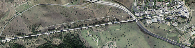
Physicists use particle accelerators to study subatomic particles and their interactions. These accelerators verify the above mass increase formula every time they are turned on. One such accelerator, located at Stanford University in California, has accelerated electrons so that they become 40 times more massive than protons, 80,000 times more massive than electrons normally are. Note that normally electrons have a mass of one two thousandth (1/2000) the mass of a proton and are easily stopped by a piece of paper. The very fast moving electrons from this accelerator can pass through meters of concrete pushing many, many protons out of the way in the process. This feat would be impossible if mass did not increase with very high velocity. Incidentally, these electrons were traveling at 99.97% the speed of light when they emerged from the accelerator.

Fig. 10.3. Aerial photograph of the 2 mile long electron accelerator at Stanford University.

Parallel and transverse force and mass

Occasionally we use the words parallel and transverse mass to emphasize the fact that it is harder to accelerator a high speed particle in the direction of its motion than it is to accelerate it perpendicular to its motion.

We can understand this by considering the relativistic form of Newton's second law of motion:

   .    (10.11)

Note that in the above equation, (10.11), the bold faced variables are vectors, a shorthand notation for all the components of a vector to be treated together: all to be multiplied by m or all to have their time derivative taken.

The time derivate of γ is done as follows:

   ,    (10.12)

where we have used the following:

   .    (10.13)

In the above equation, v⋅v represents the dot product between the vector v and itself (which yields the magnitude of v squared.)

Substituting (10.12) into (10.11) yields:

   .    (10.14)

Case I, transverse force

In the case of force applied perpendicular to the direction of motion (perpendicular to the trajectory of the particle to bend its trajectory), the first term in (10.14) is zero because v is perpendicular to dv/dt making the dot product zero. Or alternately, in this case the magnitude of velocity is not changing, making dγ/dt zero. With either argument, we are left with only the second term in (10.14), giving us:

   .    (10.15)

Case II, parallel force

In the other case, when the force is applied in the same direction as the particle's velocity to speed up the particle, then both terms of (10.11) are present. The dot product in the first term is equal to the magnitude of the two vectors. Since all three vectors in that term are in the same direction, we can use any one of them to indicate the vectorial direction of the term. We choose dv/dt to be the vector and the other two vectors (the v's) to be scalars. The force equation (10.14) written out becomes:

   .    (10.16)

We see that the parallel force increases with the cube of γ whereas the transverse force increases linearly with γ. Some put the γ³ dependence into an effective mass as:

   .    (10.17)

This allows use of the simple second law of motion with an enhanced mass:

   .    (10.18)

Transforming mass

We have derived the equation (10.5) in the rather special case shown in Fig. 10.1 above involving two identical particles. Equation (10.5), however, is very general and preserves momentum conservation in collisions of a slowly moving objects and rapidly moving ones, with equal and with unequal masses. This we will demonstrate at the end of this chapter.

In this section, we will derive a transform that relates the mass of an object moving at one relativistic velocity,  u , to its mass when it is moving at another relativistic velocity,  u' . We will work in the unprimed and the primed reference frames. In both frames the object is moving, but with different velocities. Using (10.5) we can relate the mass in each reference frame to the object's proper mass (mass when it is stationary):

   and       .

Dividing one equation by the other and solving for the unprimed mass yields:

     .     (10.19)

We now wish to simplify this a little. Most of the difficult calculation for this is the calculation of the denominator which we wish to express in terms of u instead of u'. We can do the velocity transforms using the equations from Chapter 9.

    ,       (10.20)

where γ is dependent on the relative velocity V between the reference frames themselves (not between the objects in the two frames) and is given by:

    .     (10.21)

Substituting (10.20) back into (10.19) yields:

    .     (10.22)

This can be alternately expressed in terms of the x component of the momentum p_x as:

    .     (10.23)

Comparing this with the setup (Fig. 10.1) used to derive (10.4), we see that to go from Fig. 10.1b (the unprimed frame) to Fig. 10.1c (the primed frame), that for the blue particle the unprimed x momentum is zero, making (10.23) become in this case  m' = γm. This is consistent with (10.4) because the red mass of Fig. 10.1b should be the same as the blue mass of Fig. 10.1c due to symmetry.

Transforming momentum

We actually used momentum conservation to derive the mass increase with speed in the first part of this chapter. We now want to formalize the transformation equations for momentum itself.

Momentum p is simply the mass of an object times its velocity, i.e.  p = mu , where m is the object's mass. We use the velocity transformations (9.4) along with the mass equation (10.23) to arrive at:

   .    (10.24)

Summary - momentum/mass transforms

We put (10.23) and (10.24) together, as is common:

.    (10.25)

We see that the momentum and mass transforms fit together in special relativity much the same as space coordinates and time do. In fact many graduate level textbooks on this subject really just assume (10.5), i.e.  m = γm₀ , in order that momentum and mass transforms result in the nice arrangement shown in (10.25), similar to the Lorentz transform for space and time. This allows the elegant treatment of special relativity using four-vectors, a concept that we will very briefly summarize in Chapter 14. We might emphasize that the derivation of (10.5) done at the beginning of this chapter is not technically rigorous. It uses a special collision to suggest that (10.5) would be a nice way to restore momentum conservation for such collisions.

Below we check whether the mass transform we "derived" above in fact does restore momentum conservation in the case of a general collision involving objects of differing masses and with some energy loss (partially elastic).

Checking for momentum conservation in the case of a general collision

	Galilean velocity transforms:  v'x = vx − V  vy' = vy  vz' = vz  m' = m	Lorentz velocity transform:
Fig. 10.4a. A general two body collision with arbitrary angles and velocities. The two masses,  m1  and  m2 , are of unequal size. The collision is partially elastic (some energy is lost). The initial velocity of  m1  is v1i and its final velocity (after the collision) is v1f. The initial velocity of  m2  is v2i and its final velocity (after the collision) is v2f.	Fig. 10.4b. These are the transforms for velocity for everyday life. The only change in an object's apparent velocity (in changing reference frames) is the addition or subtraction of the reference frame's velocity.	Fig. 10.4c. These are the transforms for very high speed motion, near the speed of light. These transforms are considerably more complex than the Galilean velocity transforms shown to the left.  γ  is defined as:

In this section we check if momentum conservation is upheld upon change of reference frame in the case of a general collision of two objects, objects that have different masses and lose some of their energy during the collision. A diagram of such a collision is shown in Figure 10.4a. The equations for the momentums before and after the collision are:

p_initial = m_1iv_1i + m_2iv_2i            p_final = m_1fv_1f + m_2fv_2f      .      (10.26a)

We will assume that momentum is conserved before collision, i.e. that p_initial = p_final:

m_1iv_1i + m_2iv_2i = m_1fv_1f + m_2fv_2f     (assumed).    (10.26b)

and endever to show, with this assumption, that momentum is still conserved after we change reference frames (to the primed frame), i.e. that p'_initial = p'_final , or to show:

m'_1iv'_1i + m'_2iv'_2i = ? m'_1fv'_1f + m'_2fv'_2f     (to be shown).    (10.26c)

We first do the checking using Galilean transformations, shown in Figure 10.4b (reproduced here just below).

Galilean velocity transforms:

v'x = vx − V  vy' = vy  vz' = vz  m' = m

Fig. 10.4b

I. Using Galilean transforms:

In low speed velocity transforms, the masses of the colliding objects do not change as a result of the collision, so:

m_1i = m_1f = m₁     and     m_2i = m_2f = m₂     (10.26d)     .

We'll only transform the x components of the velocities because the y and z components of velocity don't change as indicated in Fig. 10.4b. The new x components (before and after collision) of momentum in the transformed reference frame are:

Substituting in for the primed velocities from the Galilean transforms of Fig. 10.4b, we get:

   .    (10.27a)

Using (10.26b) above, we can change the last line of (10.27a) into:

   .    (10.27b)

This shows that the final momentum still equals the initial momentum when we change reference frames using Galilean transforms.

Note that the above mathematics uses the Galilean velocity transformations which are not consistent with the speed of light being invariant under changes in moving reference frames.

We next see if momentum is conserved in a new reference frame when we use Lorentz velocity transformations. Lorentz velocity transformations are shown in Fig 10.4c and reproduced just below.

Lorentz velocity transforms:

Fig. 10.4c

II. Using Lorentz transforms:

We start again with (10.26a). We then transform only the velocities, naively hoping the masses can stay the same:

   .    (10.28)

With all the complicated denominators in (10.28) there is no way to factor the two lines to make them the same.

So we see that if mass does not change with reference frame, i.e. speed, then the transformed momentum equations become a tangle that will not preserve momentum conservation.

We now add the relativistic mass transform (10.22):

m' = γm(1 − v_xV/c²)      .     (10.29)

We also need to distinguish between the mass of each object before collision and after collision, since the masses will change along with the change in velocities before and after a collision.

Substituting (10.29) into(10.28) yields:

   .    (10.30)

If we examine the factors in (10.30) we see that we can cancel out all the troublesome terms to yield the simple results:

(10.31a)

    (10.31b)

Using (10.26a), (reproduced here)

p_initial = m_1iv_1i + m_2iv_2i            p_final = m_1fv_1f + m_2fv_2f     (10.26a)      ,

allows (10.31a) and (10.31b) to be further reduced to:

    (10.31c)

    (10.31d)

The the last terms in the x components of (10.31c) and (10.31d) are linked to relativistic energy conservation. In the next chapter, we derive the famous relation that energy  E = mc² , i.e. that energy and mass are proportional. If we assume that the total relativistic energy before the collision equals the energy after the collision then

 m_1i + m_2i = m_1f + m_2f       (10.32)     ,

If we substitute momentum conservation in the initial frame (i.e. Equation (10.26b) or p'_initial = p'_final ) and also (10.32) both into (10.31d), we get:

    (10.33)

Thus momentum is conserved in the second (i.e. the primed) reference frame, as long as we assume relativistic energy conservation, i.e. (10.32).

Note that relativistic energy will be conserved even when kinetic energy is not. A collision can lose kinetic energy to heat, but if the heat is contained inside the colliding objects, it will cause them to be heavier than they otherwise would be as given by  E = mc²  where the energy E also include the kinetic energy due to the thermal vibrational motion of the atoms in each colliding object. Thus relativistic energy (and momentum conservation) will be maintained, even for partially (or totally) inelastic collisions. On the other hand, if electromagnetic radiation is given off during the collision, then the energy and momentum of this radiation needs to be factored into the energy and momentum conservation equations so that energy and momentum conservation is maintained.

all topics by author

introduction to relativity

contents of mathematics of relativity

previous: transforming velocities

next: relativistic kinetic energy